Multiple-choice data usually reach a model as right or wrong. The IRW’s nominal tables keep the option chosen. Does knowing which wrong answer a respondent picked help predict how they answer items we have not seen? We compare a 2PL on the 0/1 scores with the nominal and nested logit models on the options, out of sample, using the InterModel Vigorish (IMV), first for right/wrong, then for the option chosen and for which wrong answer.
Published
November 10, 2026
Note
This vignette — including the dataset search, the compute script, the analysis design, and the writing below — was produced largely by Claude (Anthropic), working from a task specification and with human review. Treat the methodological choices and interpretations accordingly, and check the compute script (nominal_imv_compute.R) directly if you’re relying on the numbers here.
TipThe full analysis
This page is a compact version of the comparison in Rivadeneira Quintero et al. (2026), a PsyArXiv preprint. The paper runs it on 116 of the 140 tables of irw_nominal version 5.0, ENCCEJA included, and on TIMSS, PIRLS and Czech national exams. It reports the nominal model’s gain over the 2PL in predicting the option chosen, in \(\omega_c\) and in bits split into right/wrong and which wrong answer, where on the ability scale that gain lies, and how well each model’s scores track ability against an external criterion.
Motivation
Score a multiple-choice item 0/1 and two respondents who both got it wrong look the same, though one may have chosen the answer a nearly-right reader would choose and the other an answer nobody who understood the item would pick. The course lesson on nominal models shows that the wrong answers carry information about the respondents who miss items. It leaves open whether that information improves prediction. This page asks that across the multiple-choice tables in the IRW’s nominal source, in two forms:
Right or wrong. Does a model that has seen which wrong answers a respondent chose predict better whether they will get an unseen item right?
Which option. Does it predict better which option they will choose, and in particular which wrong answer, given that they miss?
The IMV has been used on this site to ask the same kind of question about other information beyond the 0/1 scores. Response time and accuracy asks how much response times add to predictions of correctness over ability alone, and Guessing in multiple-choice data asks, on several of the same ENEM tests, whether modelling guessing helps out of sample. Calculating IMV values walks through the basic computation.
Data and methods
Dataset selection
Code
cands <-c(paste0("enem_2013_1mil_", c("ch", "cn", "lc", "mt"), "_nom"), # one ENEM test per area"wilmer-rmet-normative-data-set-2022_nom", "borges_brazil_residency_2024_pbt_nom","choi_2020_ednet_listening_nom", "vocabulary_iq_nom", "psychtools_ability_nom"# ... and every other table with at least 10 items in irw_nominal v3.3)
The candidates are four ENEM tests, one per subject area from 2013, and every other table with at least 10 items that irw_nominal held at version 3.3 (October 1, 2026): 32 tables in all, listed by hand in the compute script because the nominal metadata lags behind releases. The 56 ENCCEJA tables added in version 4.1 are not among them. A table is analysed if it is single-answer multiple choice: one keyed option per item, and no item with more than 12 answers each chosen by at least 1% of respondents or with its rarer answers together making up more than 10% of responses. Each table is fitted on 10 independent draws of up to 3,000 respondents.
Blanks and rare options. ENEM codes a blank as a dot (.) and a double mark as an asterisk (*). These are not options, so those responses are dropped first. A wrong option chosen by fewer than 1% of respondents is then pooled with the item’s other rare options, and if the pooled group is still under 1%, those responses are dropped too. Left to that rule, blanks and double marks would enter the option models as a distractor, alone or pooled with rare options, on any item where they reach 1% of responses. On some recent ENEM tests they do on many items: 14 of the 44 in the IRW’s 2023 math table, across all its respondents. Respondents left with fewer than half the items are dropped, and so is any table with fewer than 1,000 respondents remaining.
Sparse tables. Some tables come from adaptive or self-paced systems, where each respondent sees a small part of a large item bank: EdNet’s TOEIC practice app, for example. There we keep a dense block: the 40 most-answered items, and the respondents who answered at least half of them. These items are not a random draw from the bank, so the result describes the block. Such tables are marked † below.
Models
Three item response models are fitted to every table, with the Rasch model alongside as a reference point.
2PL. The usual model for right/wrong. It sees only the 0/1 scores.
Nominal response model(Bock 1972). Every option, the key included, gets its own slope and intercept on θ. The probability of option \(k\) is a softmax over the options’ linear predictors.
Nested logit(Suh and Bolt 2010). A 2PL for the key, and a nominal model among the distractors for the respondents who miss. The key’s curve keeps the 2PL’s shape; the wrong answers only add information about who misses the item and how.
The course lesson walks through both option models on one test; this page does not re-derive them.
How the nominal model is fitted.mirt’s default writes each option’s slope as a common slope \(a_1\) times an option weight, with the weights of two options fixed. We fix \(a_1\) at 1 instead and leave every option’s slope free except the reference option’s. This is the same model, written without the product. The difference is in where mirt’s EM stops. On these data the default’s EM drifts toward a small \(a_1\) with large option weights and moves so slowly there that it meets mirt’s tolerance before the maximum. In the first draw of each table (60 folds in all), the default parameterization ended a median of 14.8 log-likelihood units below the one used here (up to 291), while reporting convergence every time. Both are fitted to the same training cells, so the gap is the default stopping short, not a different model.
Per-table computation
For each candidate table, fit_one() in the compute script:
Fetches the table with irw_fetch(source = "nom"), keeps one response per person and item, keeps a dense block if the table is sparse, and takes 10 independent draws of up to 3,000 respondents. Steps 2 to 5 run once per draw.
Builds two person × item matrices, one holding the option chosen (with the key coded as the last category) and one holding the 0/1 score. Blanks are dropped, rare options are pooled, and thin items and respondents are dropped, as described above.
Splits the observed person-item cells at random into five folds. For each fold, it fits the Rasch model and the 2PL to the 0/1 scores, and the nominal model and the nested logit to the options, using mirt with all the fold’s cells hidden.
Takes each model’s EAP θ, estimated from the visible cells, and predicts every hidden cell. It records P(key) and the probability of every option.
Computes the three IMVs described below: over all held-out cells together, for each fold on its own, and within thirds of the 2PL θ.
The results are then averaged over draws, with standard errors from the draw-to-draw spread.
Code
fit_draw <-function(n, d) { # one draw of up to 3,000 respondents P <-prep(n) # options (key last) and 0/1 matrices, blanks dropped fold <-sample(rep_len(1:5, length(obs))) # folds over observed person-item cells per_fold <-lapply(1:5, function(k) { opt_tr <- opt; opt_tr[obs[fold == k]] <-NA# hide this fold x_tr <- x01; x_tr[obs[fold == k]] <-NA mods <-list(rasch =mirt(x_tr, 1, "Rasch"),twopl =mirt(x_tr, 1, "2PL"),nominal =mirt(opt_tr, 1, "nominal", pars =nominal_pars(opt_tr), # a1 fixed at 1technical =list(NCYCLES =2000)),nested =mirt(opt_tr, 1, "2PLNRM", key = ncat, technical =list(NCYCLES =2000)) )# Each model's EAP theta -> P(key) and every option's probability on the hidden cells.# Rasch and the 2PL split 1 - P(key) by the training-cell distractor shares. })# imv.binary() on right/wrong; omega_c on the option chosen and on which wrong answer}fit_one <-function(tn) { draws <-readRDS(draws_file(cache_dir, tn)) # N_DRAWS samples, taken in fetch_one() per_draw <-lapply(seq_along(draws), function(d) fit_draw(draws[[d]], d))# means over draws, and standard errors from the draw-to-draw spread}
Of the 32 candidate tables, 12 produced usable results. The rest are listed, with the reason, under Table 1. In 1 of the 2,400 fold fits (1 nested logit fit), EM stopped before mirt’s convergence criterion; we use that fit as it stands.
Note
To reproduce with current IRW holdings, clear the caches described under Reproducibility, re-run nominal_imv_compute.R and commit the updated nominal_imv_data/nominal_imv_results.rds.
Three versions of the IMV
The InterModel Vigorish compares two models’ out-of-sample predictions. For binary outcomes it converts each model’s mean log-likelihood on the held-out cells into a weighted coin: the coin whose own expected log-likelihood equals the model’s. If a model’s predictions are as good as betting on a coin that lands heads with probability \(w\), the IMV of model 1 over model 0 is the relative gain in that weight, \((w_1 - w_0)/w_0\). We write A → B for the IMV of model B over model A. The Rasch → 2PL gain on the same cells is our yardstick: the value of letting items differ in discrimination, which most analysts already consider worth having.
1. Right/wrong (binary IMV). Every model predicts P(key) on the hidden cells, and imv::imv.binary() compares them. All four models are judged on the same outcome.
2. The option chosen (\(\omega_c\)). Here the outcome is which of the item’s options the respondent chose, and the IMV is \(\omega_c\), the polytomous IMV of Kanopka (2023, ch. 3). It is built from binary bets. For every pair of options on an item, it takes the held-out cells where one of the two was chosen and computes an ordinary binary IMV for which of the two it was, from each model’s probabilities of those two options rescaled to sum to one. The pairwise IMVs are averaged within an option, weighting by how many cells each pair has, and then across options, weighting by how often each option was chosen on the item’s cells. We compute it per item on all the held-out cells of a draw and average it over items. Because every piece is a binary IMV, \(\omega_c\) is on the binary IMV’s scale whatever the number of options, so tables with different numbers of options can be set side by side. An \(\omega_c\) of 0.02 means that, averaged over pairs of options, the model’s bet on which of the two was chosen matches a coin whose weight is about 2% higher than the baseline’s.
A 2PL predicts only P(key), so to enter this comparison it needs a rule for the wrong options. We use the simplest: 2PL + shares. The 2PL gives P(key), and 1 − P(key) is split among the wrong options in the proportions in which they were chosen on that item’s training cells. That baseline already knows which distractors are popular. What it lacks, and what the option models add, is any link between θ and the choice of distractor.
3. Which wrong answer. The third version keeps only the held-out cells answered wrongly and computes \(\omega_c\) over the pairs of wrong options. A model’s probabilities of two wrong options, rescaled to sum to one, do not depend on its P(key), and for the 2PL + shares baseline they are just the two options’ shares, so this IMV measures one thing: how much knowing θ tells you about which wrong answer someone picks. Items are averaged weighting by their held-out wrong answers, so an easy item with a few dozen of them counts less than a hard one with hundreds.
Results
Does knowing the wrong answers predict right/wrong better?
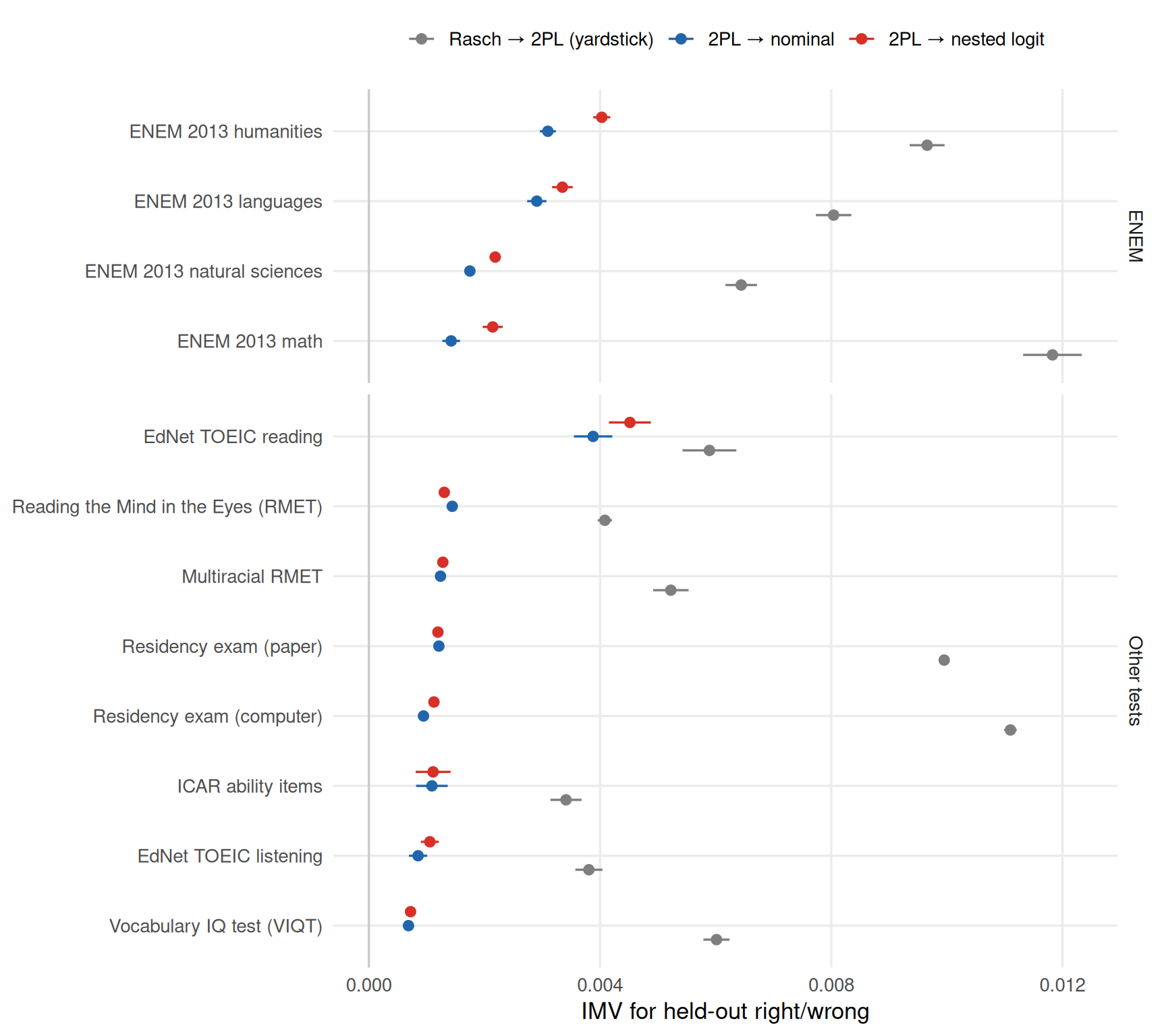
All three comparisons in Figure 1 are the same bet: on each held-out cell, which model gave the better probability that the respondent chose the key? Each model makes that prediction from its own θ, estimated from the respondent’s visible cells. The 2PL and Rasch read P(key) straight off their item curves. The nominal model and the nested logit predict a probability for every option, and we keep only the key’s; all the wrong options together make up “incorrect”. So the option models are scored on right/wrong exactly as the 2PL is.
Moving from the 2PL to an option model changes two things at once:
θ. The option models estimate θ from which wrong answers a respondent chose, not just whether they were wrong, so two people with the same score can get different θs.
The key’s curve. In the nominal model the key is one category of a softmax over all the options, so its curve depends on every distractor’s slope and intercept and need not have the 2PL’s shape. The nested logit keeps the 2PL’s curve for the key and uses the distractors only below it.
So the red dot (2PL → nested logit) is close to the value of the better θ alone. The blue dot (2PL → nominal) is the better θ plus whatever re-drawing the key’s curve adds or costs. The gap between them is the price, or payoff, of that new curve.
Figure 1: Out-of-sample binary IMV for three model comparisons. Grey: Rasch → 2PL, the yardstick. Blue: the nominal model changes both θ and the key’s curve. Red: the nested logit changes θ but keeps the 2PL’s curve for the key. Points are means over draws; bars are ±2 standard errors across draws.
Knowing which wrong answers a respondent chose elsewhere always helps, but only a little. The nested logit beats the 2PL on all 12 tables and in 583 of the 600 folds across all draws, with IMVs from 0.0007 to 0.0045. Every one of those is smaller than the Rasch → 2PL gain on the same cells.
Points are means over the draws and bars are ±2 standard errors across them. Each draw has its own sample of respondents and its own random split into folds, so the bars reflect both. Residency exam (paper) and ICAR ability items have no more than 3,000 respondents, so they use all of them in every draw and their bars reflect the split alone. The median standard error of 2PL → nested is 0.00006. Where the bars of two tables overlap, read the difference between them as a tie. Two models on the same table share draws and folds, so the difference between them is usually more precise than their bars suggest.
The nested logit also matches or beats the nominal model on 10 of the 12 tables. The exceptions are Reading the Mind in the Eyes (RMET) and Residency exam (paper). Only on Reading the Mind in the Eyes (RMET) is the nominal model’s lead beyond two standard errors of the paired difference. Elsewhere, blue sits at or left of red, so re-drawing the key’s curve mostly costs accuracy rather than adding it. The cost, relative to what the nested logit gains, is largest on ENEM 2013 math, at 34%. For predicting right and wrong, the better way to use the distractors is to let them inform θ and leave the key’s curve alone.
How far red gets toward grey varies a lot. The nested logit’s gain is 77% of the Rasch → 2PL gain on EdNet TOEIC reading but only 10% on the Residency exam (computer). The “Nested ÷ yardstick” column of Table 1 gives it for every table; it has no clear relation to how hard the test is. It is lowest on the two residency exams and the VIQT, at about a tenth of the yardstick. The residency exams are the longest tests here, at around 100 items, so for them a likely reason is that θ is already well estimated from the right/wrong scores alone, leaving the distractors little to add.
Does it predict which option is chosen?
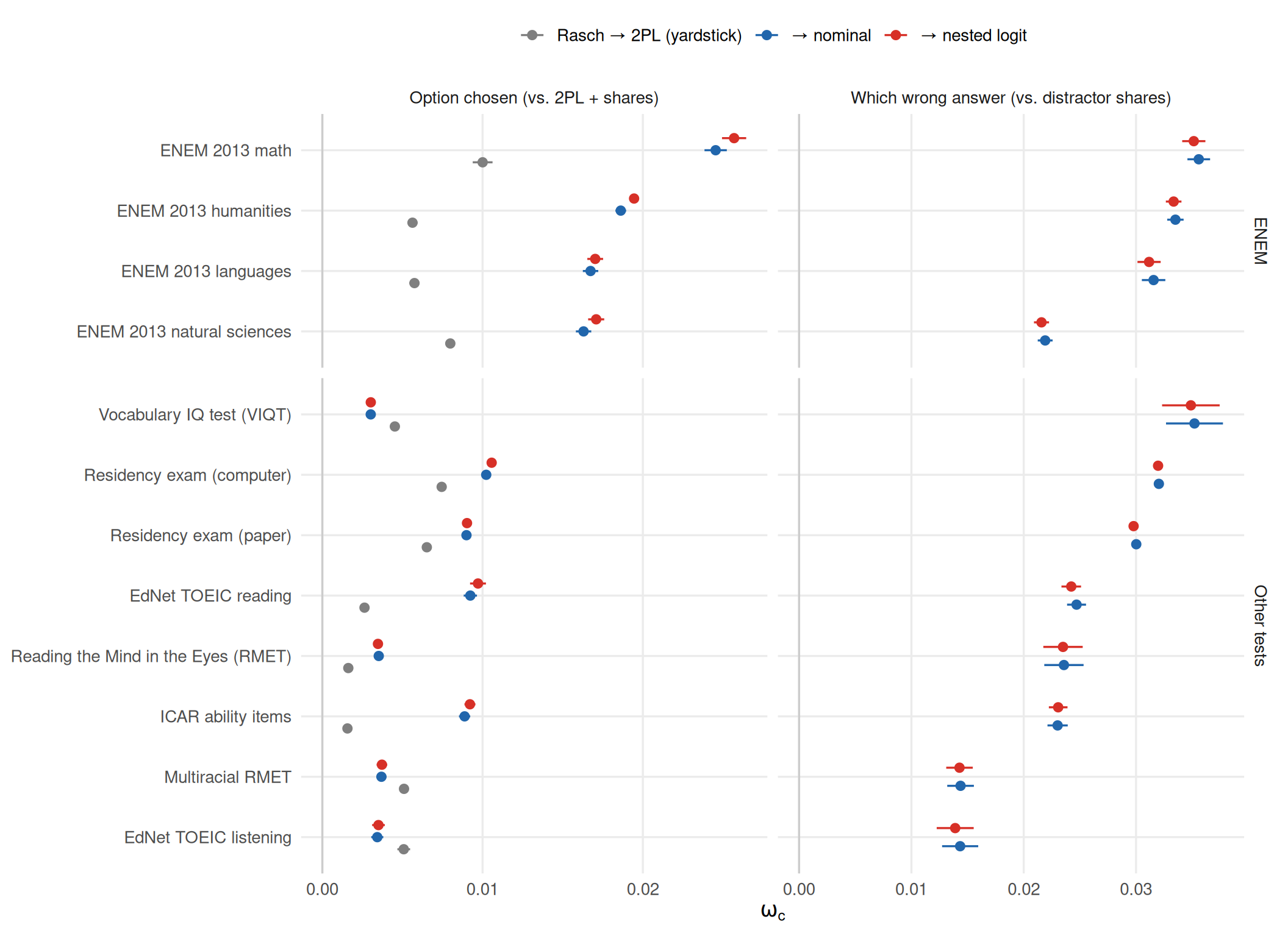
Now the bet changes. Instead of right or wrong, the outcome on each held-out cell is the option chosen, scored with \(\omega_c\). The 2PL and Rasch enter with the “+ shares” rule: their P(key), with the rest split among the distractors by how popular each was on the training cells. Grey is again the yardstick, here the Rasch → 2PL gain measured with \(\omega_c\). The left panel of Figure 2 scores every held-out cell; the right panel, described below, scores only the wrong answers.
Figure 2: Out-of-sample \(\omega_c\). Left: the option chosen on every held-out cell, with 2PL + shares as the baseline for the option models. Right: which wrong answer was chosen, over held-out wrong answers only, with the distractors’ training shares as the baseline. Points are means over draws; bars are ±2 standard errors across draws. The two panels have different x-axis ranges.
Judged on the option chosen, the option models beat 2PL + shares on every table. That is not guaranteed, because the baseline already knows how popular each distractor is. Grey is not a like-for-like yardstick here, though. Rasch and the 2PL split the wrong answers by the same shares, so adding discrimination can gain only on the pairs that include the key. \(\omega_c\) averages over all pairs, so how the two gains compare depends on how the pairs are weighted. The paper (Rivadeneira Quintero et al. 2026) compares them in bits instead, where the nominal model’s gain over the 2PL exceeds the Rasch → 2PL gain on 89 of its 116 tables.
That gain mixes two things: predicting the key better, which the first section already measured, and predicting which distractor is chosen. The right panel of Figure 2 isolates the second. It keeps only the held-out cells answered wrongly and asks which wrong answer was chosen. The baseline is the distractors’ shares alone, which know nothing about θ, so this IMV measures what knowing θ tells you about the choice of distractor. Rasch and the 2PL use the same shares there, so the yardstick is zero and the right panel has no grey.
Among held-out wrong answers, θ predicts which one was chosen on every table, with \(\omega_c\) from 0.0139 to 0.0351. These values are not set against the right/wrong IMVs above: the outcome is different, and the baseline’s predictions for a pair of distractors are often close to 50/50, where the IMV’s scale moves fastest (see Limitations). The nominal model and the nested logit come within 4% of each other on every table, as expected, since both model the choice among distractors the same way. In the first section the nested logit could use the wrong answers only through θ, and θ is already well estimated from the scores; that is a likely reason its gains there are small.
Who gains?
The next two figures split the held-out cells into thirds of the 2PL θ and compute each IMV within each third. Each line is one table. Click a line, or choose a table from the menu above the figure, to pick it out from the rest; double-click to clear. Hover over a point for its table and value.
Code
terc_plot("twopl_to_nest", "IMV, 2PL → nested logit", "Pick out a table")
Figure 3: Binary IMV, 2PL → nested logit, within thirds of the 2PL θ. One line per table: means over draws, with bars of ±2 standard errors across draws. Red lines are the four ENEM tests and blue lines the other tests: here colour marks the test, not the model.
For right/wrong, where the gain lands depends on the test. On most tables it goes to the bottom third, as the course lesson’s information curves predict: low scorers are the respondents with wrong answers to read. ENEM never shows that pattern. On humanities and languages the gain peaks in the middle third. On the two hardest tests (natural sciences and math, about a quarter of responses correct), it rises toward the top, and the bottom third gains least. Low scorers who guess close to at random would produce this pattern, because their wrong answers carry no signal. Issue #284 tests this directly. The paper finds that ENEM’s low scorers do not spread their wrong answers evenly over the distractors, and that in ENEM a large part of what the options add at the bottom of the scale is also captured by the 3PL’s guessing floor.
Code
terc_plot("wrong_shares_to_nest", "ω<sub>c</sub>, shares → nested logit", "Pick out a table ")
Figure 4: Which wrong answer: \(\omega_c\), shares → nested logit, over held-out wrong answers within thirds of the 2PL θ. One line per table: means over draws, with bars of ±2 standard errors across draws. Red lines are the four ENEM tests and blue lines the other tests: here colour marks the test, not the model.
For which wrong answer, the middle third gains least on every table. Beyond that the ends differ. On the two hardest ENEM tests, natural sciences and math, the top third gains most and the bottom third much less, as near-random guessing at the bottom would predict. On the VIQT and the multiracial RMET it is the top third that gains little, within two standard errors of the middle. The paper (Rivadeneira Quintero et al. 2026) measures this differently, in bits per wrong answer, for the nominal model against the 2PL with overall distractor shares, by decile of the 2PL θ, on all 116 of its tables: the curve is U-shaped in ENEM, ENCCEJA and the other tests alike, the median gain is largest in the top decile in each, and the maximum falls in the top decile in 104 of the 116 tables. Thirds are much coarser than deciles, and \(\omega_c\) rescales and averages over pairs of options, so the two need not agree table by table. The dip in the middle is partly built in. The shares are the distractors’ popularity averaged over everyone who missed, so they describe a typical wrong answer, from the middle of the distribution, best. The rest is the nominal model’s crossing option curves at work. If low scorers who miss are drawn to one distractor and high scorers who miss to another, then knowing which end of the scale a respondent sits at tells you which to expect. Which distractors those are, and why they pull, is the question of issue #285.
Table 1: The twelve analysed tables. N is the respondents in a draw after cleaning, averaged over draws; Items is the count in the first draw.
Table
N
Items
% correct
Rasch → 2PL
2PL → nested (SE)
Nested ÷ yardstick
Option: 2PL + shares → nested
Wrong answer: shares → nested
ENEM 2013 humanities
3,000
45
38%
0.0097
0.0040 (0.00007)
42%
0.0195
0.0333
ENEM 2013 languages
2,996
50
42%
0.0080
0.0033 (0.00009)
42%
0.0170
0.0312
ENEM 2013 natural sciences
2,996
45
26%
0.0064
0.0022 (0.00005)
34%
0.0171
0.0216
ENEM 2013 math
2,994
45
27%
0.0118
0.0021 (0.00009)
18%
0.0257
0.0351
EdNet TOEIC reading †
2,998
40
54%
0.0059
0.0045 (0.0002)
77%
0.0097
0.0242
Reading the Mind in the Eyes (RMET)
3,000
36
71%
0.0041
0.0013 (0.00003)
32%
0.0035
0.0235
Multiracial RMET
2,994
37
64%
0.0052
0.0013 (0.00004)
24%
0.0037
0.0143
Residency exam (paper)
1,994
98
59%
0.0100
0.0012 (0.00002)
12%
0.0090
0.0298
Residency exam (computer)
2,991
118
56%
0.0111
0.0011 (0.00002)
10%
0.0106
0.0320
ICAR ability items
1,469
16
51%
0.0034
0.0011 (0.0002)
33%
0.0092
0.0231
EdNet TOEIC listening †
3,000
40
58%
0.0038
0.0011 (0.00008)
28%
0.0035
0.0139
Vocabulary IQ test (VIQT)
2,780
37
82%
0.0060
0.0007 (0.00002)
12%
0.0030
0.0349
† A dense block of a sparse table: the 40 most-answered items and the respondents who answered at least half of them. Every IMV is a mean over draws; the standard error over draws is in parentheses. The last two columns are \(\omega_c\); the others are the binary IMV.
Code
reason <-function(x) dplyr::case_when(grepl("^N = ", x) ~"Fewer than 1,000 respondents",grepl("^sparse design", x) ~"Sparse design with no dense block (each respondent saw a small part of a large item bank)",grepl("option set changes", x) ~"Option set changes from one presentation of an item to the next (adaptive practice)",grepl("free text|not one keyed|resp is not 0/1|no resp/text", x) ~"Not single-answer multiple choice (free text, typed numbers, multi-select, or unscored)",grepl("MIN_ITEMS", x) ~"Fewer than 10 usable items (an item needs at least two wrong answers each chosen by 1% or more)",TRUE~ x)# vapply, not sapply: with no skipped table (a TABLES or PILOT run), sapply()# returns list() and case_when() fails.sk <-tibble(table =vapply(skipped, `[[`, character(1), "table"),why =reason(vapply(skipped, `[[`, character(1), "skipped")))# ASAP 2.0 is essays, one of seven prompts per student: free text, not a sparse item bank.sk$why[sk$table =="asap20train_nom"] <-reason("free text")cat("**Not analysed.** Four tables have fewer than 10 items and were not attempted (`cos101_2026`, ","`goldberg_2018_spa_computer_use`, `himmelstein-berlin_numeracy-2025`, `mthimkhulu_2023_pirls_reading`).",if (nrow(sk)) " The other candidates were tried and set aside:\n\n"else"\n\n", sep ="")
Not analysed. Four tables have fewer than 10 items and were not attempted (cos101_2026, goldberg_2018_spa_computer_use, himmelstein-berlin_numeracy-2025, mthimkhulu_2023_pirls_reading). The other candidates were tried and set aside:
Sparse design with no dense block (each respondent saw a small part of a large item bank): zorowitz_2023_marsib, suarez_2026_statistics, semeval2013_scientsbank
Not single-answer multiple choice (free text, typed numbers, multi-select, or unscored): fitz_2024_numeracy, voropaeva_2026_health_media, preference_inventory, much_tte_2025_matrixreasoning, asap20train, persuade_learningagency
Fewer than 1,000 respondents: experimental_iq, myszkowski_2018_spmls, nomt_hooper_2024_study2, blum_2018_imak
Fewer than 10 usable items (an item needs at least two wrong answers each chosen by 1% or more): sirota_2018_crt, cifar10h, hachenberger_2025_stroop_main, hachenberger_2025_stroop_pilot, much_tte_2025_concentrationtask
Option set changes from one presentation of an item to the next (adaptive practice): papousek_2017_anatomy, geography
Limitations
Draws of 3,000 respondents. Each draw takes up to 3,000 respondents, and the results average 10 independent draws, each with its own split into folds. On tables much larger than 3,000 the draws barely overlap, so the spread between them is close to what fresh samples would give. On smaller tables the draws share respondents, so the standard errors mostly reflect the split and understate the uncertainty from sampling respondents.
Four ENEM tests stand in for 52, and ENCCEJA is left out. We used one 2013 test per subject area. The differences between areas are large here; whether they hold in other years is untested. The 56 ENCCEJA tables, added to irw_nominal after this analysis was designed, are not included. The paper (Rivadeneira Quintero et al. 2026) runs the comparison on 116 of the 140 tables of version 5.0, all 52 ENEM and 56 ENCCEJA tables among them.
Dense blocks are not random samples of items. For EdNet, the 40 most-answered questions and the learners who answered at least half of them are a particular slice of the app’s use. The EdNet results describe that block, not the whole item bank.
Rare answers are pooled or dropped. Options chosen by fewer than 1% of respondents are pooled, and ENEM’s blanks and double marks are dropped. An unusual distractor may be exactly where a wrong answer says the most, and these IMVs never score it.
The which-wrong-answer baseline knows nothing about θ. The positive IMVs in the right panel of Figure 2 show that θ is informative about which distractor is chosen. They do not show that the nominal model beats other ways of using ability, such as distractor shares computed separately by score band.
\(\omega_c\) scores a different outcome from right/wrong. It is on the binary IMV’s scale, but that scale moves fastest where the baseline’s predictions are close to 50/50, which is common for a pair of distractors and rare for the 2PL’s predictions of right and wrong. So compare models within a column, not the size of \(\omega_c\) with the size of the right/wrong IMV.
“Who gains” groups respondents by the 2PL θ. Grouping by an option model’s θ would move some respondents between thirds and could change the shape of the curves at the margins.
Only unidimensional models, and no guessing. We did not fit a 3PL or any other guessing model; the guessing vignette covers those on ENEM. The paper adds the 3PL and the nested logit with guessing: against the 3PL, the nominal model’s gain on right/wrong disappears overall and reverses on ENEM, while the nested logit with guessing beats the 3PL on right/wrong in all 116 tables.
Cross-validation is over cells, not people. The held-out cells belong to respondents whose other answers the models have seen, so these IMVs measure predicting a missing response from a known respondent. Scoring new respondents from a few items could show a different gain. The paper also scores test-takers held out of calibration, from half of their responses, and there the nominal model still improves on the 2PL in predicting the option chosen, in all 116 tables.
These results were computed against approximately IRW v626 (the corpus as of October 25, 2026).
NoteHow this version was determined
The version was inferred from when the results were computed, not recorded during the run, so it may be off by a version or more. To pin data to an exact version, use irw_use_version().
Results were computed on October 25, 2026. To regenerate, from the project root:
# A read-scoped Redivis token, for irw_fetch() and irw_save_bibtex(). Without# it, the redivis package opens a browser to log in and waits for up to 10 minutes.exportREDIVIS_API_TOKEN=...N_DRAWS=10 WORKERS=4 Rscript vignettes/nominal_imv_compute.Rquarto render vignettes/nominal_imv.qmd
The script needs the R packages irw, mirt, imv, furrr, data.table, dplyr and tibble. The results above were computed with R 4.6.0, irw 1.3.0 and mirt 1.47: each fitted table’s entry in nominal_imv_results.rds records the irw and mirt versions it used, and session holds the full sessionInfo(). renv.lock pins other versions of both, which this page does not need to render, so a run inside the renv library may not reproduce these numbers exactly.
Three environment variables control the run:
N_DRAWS (default 10): draws per table. Each draw refits all four models in five folds, so the run takes about N_DRAWS times as long as a single draw.
WORKERS (default: half the cores, at most 4): tables fitted in parallel. It does not change the results.
TABLES: a comma-separated subset of the candidate tables, to check the pipeline quickly. Its numbers will not match this page’s, because each table’s draws and folds depend on its position in the list and on the tables fetched before it. It also overwrites nominal_imv_results.rds and references.bib with only those tables, so do not commit its output; the page then shows a partial-run warning.
The full run (32 candidate tables, 12 fitted, 10 draws) took about 40 minutes with WORKERS=7 on an 18-core Mac; each table’s fitting time is stored in its seconds field. Fetching holds one ENEM table, about 3 GB, in memory at a time. As a quick check, TABLES=psychtools_ability_nom,vocabulary_iq_nom N_DRAWS=2 WORKERS=2 runs in about two minutes.
Caches and resuming. Each table’s draws are cached in ~/.cache/irw_nominal_imv/<table>_draws<N_DRAWS>.rds, with the held-out predictions under cells/, and recent versions of irw also keep their own copy of every table they download (see irw_cache_info()). Per-table results go to vignettes/nominal_imv_data/fits/<table>_draws<N_DRAWS>.rds, which is gitignored. A table with a file in fits/ is not refitted, so an interrupted run resumes where it stopped. After changing the script, delete fits/, or the old results are reused. To pick up newer IRW data, delete ~/.cache/irw_nominal_imv as well: otherwise the old draws are refitted, and the results are dated by the new run rather than by the download.
Determinism. With the same tables in the same order and the same N_DRAWS, two runs give identical results, whether or not the caches exist and whatever WORKERS is. If the fetch step is interrupted, the tables fetched after the restart are drawn from a different random state than in an uninterrupted run; to get the same draws, delete ~/.cache/irw_nominal_imv and start again.
Tip
The compute script already writes the datasets’ BibTeX, with the methods papers this page cites, to nominal_imv_data/references.bib. To get the datasets’ entries in a file of their own, from the project root after running the script:
Bock, R. Darrell. 1972. “Estimating Item Parameters and Latent Ability When Responses Are Scored in Two or More Nominal Categories.”Psychometrika 37 (1): 29–51. https://doi.org/10.1007/BF02291411.
Rivadeneira Quintero, Santiago, Klint Kanopka, Mateus Mazzaferro, and Benjamin W. Domingue. 2026. What Is a Wrong Answer Worth? The Out-of-Sample Value of the Chosen Option in Multiple-Choice Tests. PsyArXiv preprint. https://doi.org/10.31234/osf.io/zwvm2_v1.
Suh, Youngsuk, and Daniel M. Bolt. 2010. “Nested Logit Models for Multiple-Choice Item Response Data.”Psychometrika 75 (3): 454–73. https://doi.org/10.1007/s11336-010-9163-7.