The Competition Data Standard

Note: This is an experimental feature.

The data standard

The IRW competition data standard is meant to describe data derived from pairwise comparisons or competitions. Such data are widely analyzed using Elo or Bradley-Luce-Terry approaches; more information about these approaches is available here. The key distinction between these data and the conventional IRW data is that there are not id and item identifiers here but rather identifers of the two agents that are involved in a given competition.

• agent_a name/id of first competitor
• agent_b name/id of second competitor
• date Time of the data point in UNIX format.
• homefield Indicator of agent that had advantage based on game features (e.g., where game was played, who played first, etc).
• score_a Score of agent_a.
• score_b Score of agent_b.
• winner Winner of the competition (typically based on a comparison of scores). Values will be agent_a, agent_b or draw.

Additional information that may be predictive of the outcome can be included as additional columns.

Accessing the competition data

The competitions data can be accessed from both the R and Python irw packages:

R

# Install and load the package with `devtools::install_github("itemresponsewarehouse/Rpkg")`
library(irw)

# View available competition data
irw_list_tables(source="comp")

# Fetch competition data
df <- irw_fetch("collegefb_2021and2022", source="comp")
head(df)

Python

# Install package with `pip install "git+https://github.com/itemresponsewarehouse/Python-pkg.git"`
import irw

# View available competition data
irw.list_tables(source="comp")

# Fetch competition data
df = irw.fetch("collegefb_2021and2022", source="comp")
head(df)

Documentation related to the tables (including table names as with collegefb_2021and2022) can be found here.

An example

Here is a first example wherein we fit an Elo model to data from the NFL.

R

library(elo)
library(BradleyTerry2)

# Fetch and prepare data
df <- irw::irw_fetch("nfl_2010-2019", source = 'comp')
df <- df[order(df$date), ]

# ===== Elo ANALYSIS =====
er <- elo.run(score(score_a, score_b) ~ agent_a + agent_b, 
              data = df, k = 20)

# Convert Elo results to long format
elo_results <- as.data.frame(er)
elo_long <- lapply(seq_len(nrow(elo_results)), function(i) {
  data.frame(
    team = c(elo_results$team.A[i], elo_results$team.B[i]),
    elo = c(elo_results$elo.A[i], elo_results$elo.B[i]),
    date = df$date[i]
  )
})
elo_long <- do.call(rbind, elo_long)

# Convert dates to years with decimal (e.g., 2015.5 for mid-2015)
elo_long$year <- elo_long$date/(365*24*60*60)


elo_by_team <- split(elo_long, elo_long$team)

# ===== BRADLEY-TERRY ANALYSIS =====
# Create season variable based on date gaps
date_diff <- diff(df$date)
df$season <- c(0, cumsum(date_diff > 1e7)) + 2010

# Prepare data for BT model
df_bt <- df[df$winner != 'draw', ]
df_bt$win <- as.numeric(df_bt$winner == 'agent_a')
df_bt$agent_a <- factor(df_bt$agent_a)
df_bt$agent_b <- factor(df_bt$agent_b)

# Fit BT models by season
bt_by_season <- lapply(split(df_bt, df_bt$season), function(season_df) {
  mod <- BTm(win, agent_a, agent_b, data = season_df, id = "team")
  co <- coef(mod)
  names(co) <- gsub("team", "", names(co))
  data.frame(
    season = unique(season_df$season),
    est = co,
    team = names(co),
    row.names = NULL
  )
})
bt_results <- do.call(rbind, bt_by_season)
bt_by_team <- split(bt_results, bt_results$team)

# ===== PLOTTING =====
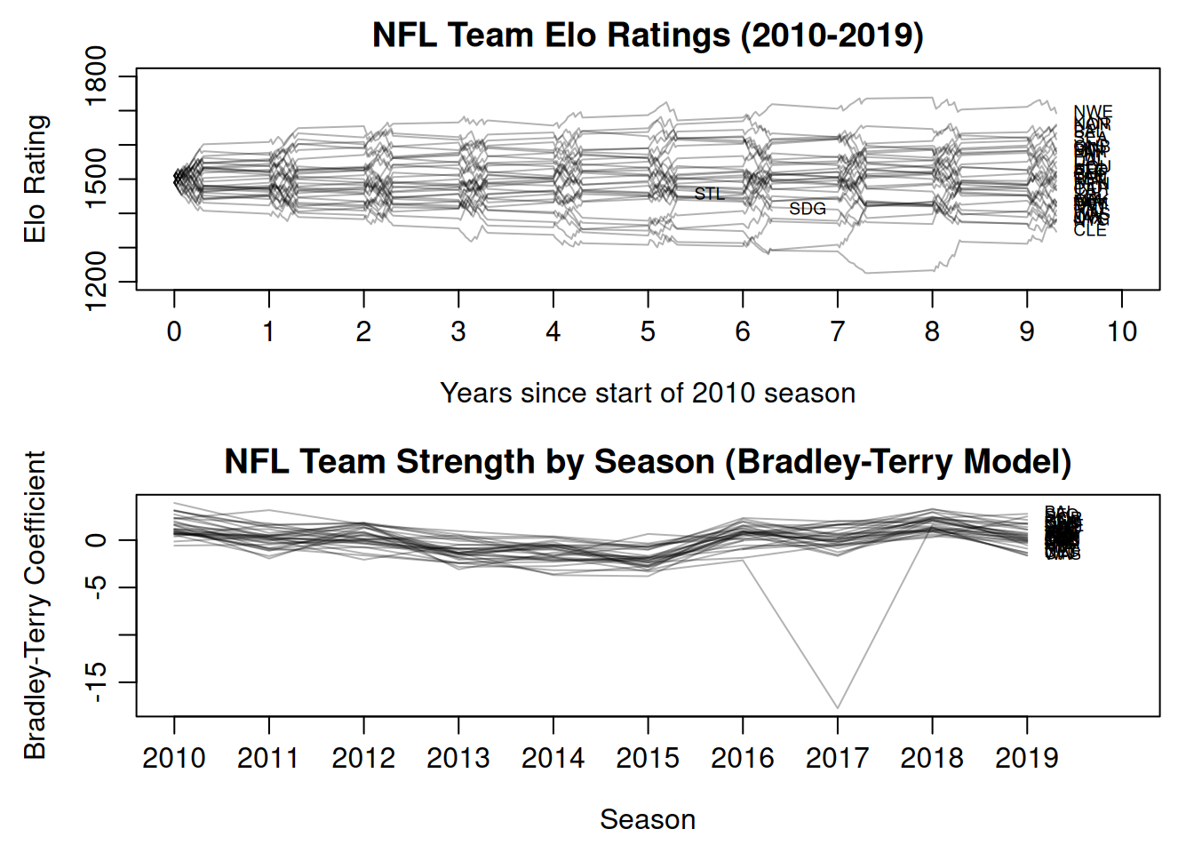
par(mfrow = c(2, 1), mgp = c(2.5, 0.7, 0), mar = c(4, 4, 2, 1))

# Plot 1: Elo ratings over time
plot(NULL, 
     xlim = c(0, 10),
     ylim = c(1200,1800),
     xlab = "Years since start of 2010 season", 
     ylab = "Elo Rating",
     main = "NFL Team Elo Ratings (2010-2019)",
     xaxt = "n")
axis(1, at = 0:10)

for (team_data in elo_by_team) {
  lines(team_data$year, team_data$elo, col = rgb(0, 0, 0, 0.3))
  n <- nrow(team_data)
  text(team_data$year[n], team_data$elo[n], team_data$team[n], 
       pos = 4, cex = 0.6)
}

# Plot 2: Bradley-Terry coefficients by season
plot(NULL, 
     xlim = c(2010, 2020),
     ylim = range(bt_results$est,na.rm=TRUE),
     xlab = "Season", 
     ylab = "Bradley-Terry Coefficient",
     main = "NFL Team Strength by Season (Bradley-Terry Model)",
     xaxt = "n")
axis(1, at = 2010:2019)

for (team_data in bt_by_team) {
  lines(team_data$season, team_data$est, col = rgb(0, 0, 0, 0.3))
  n <- nrow(team_data)
  text(team_data$season[n], team_data$est[n], team_data$team[n], 
       pos = 4, cex = 0.6)
}