Response Time and Accuracy: An IMV Analysis

How much does knowing how fast a person responded improve predictions of whether they answered correctly? We fit Rasch IRT to binary accuracy data from IRW datasets with response times, then quantify the gain from adding within-item-centered log(RT) using the InterModel Vigorish (IMV). Motivated by Domingue et al. (2022).

Published

May 20, 2026

Overview

IRT models predict binary accuracy from a latent ability estimate — but they ignore when a person responded. Response time (RT) carries its own signal about item-person fit: very fast incorrect responses may reflect guessing, while slow correct responses may reflect effortful retrieval. The question is whether RT adds predictive value over and above the IRT probability.

We answer this using the InterModel Vigorish [IMV; Domingue et al. (2022)], a log-score measure of how much one model’s predictions improve on another’s. For each IRW dataset with RT and binary accuracy, we compare three nested models:

M0: resp ~ (1|item) + (1|id) — a random-item Rasch model (De Boeck et al. 2011) with crossed random effects for item difficulty and person ability, no RT
M1: resp ~ rt_cwi + (1|item) + (1|id) — add within-item-centered log(RT), linear
M2: resp ~ spl1 + spl2 + spl3 + spl4 + (1|item) + (1|id) — add flexible spline RT

rt_cwi = log(rt) − mean_item(log(rt)) centers RT within items, isolating the micro-speed–accuracy tradeoff: is this person faster or slower than average on this item, and does that predict correctness? The random effects for item and person replace a separately-fitted Rasch model, estimating item difficulty and person ability jointly with the RT effect.

spl1–spl4 are the four columns of a B-spline basis (bs(rt_cwi, df=4)) computed from rt_cwi on the full dataset and stored as pre-computed columns. Precomputing the basis (rather than evaluating bs() inline) ensures that imv()’s internal model updates operate on the same feature matrix.

Datasets

Code

results |>
  select(table_name, N, J, n_obs) |>
  arrange(desc(n_obs)) |>
  knitr::kable(
    col.names = c("Dataset", "N persons", "J items", "Obs."),
    format.args = list(big.mark = ",")
  )

Table 1: IRW datasets used in this analysis. All have binary accuracy responses and response times.

Dataset	N persons	J items	Obs.
credentialform_lnirt	556	200	99,992
nomt_hooper_2024_study2	393	144	56,587
himmelstein-impossible_question-2025	766	90	44,996
vocab_assessment_3_to_8_year_old_children	500	47	23,500
wilmer-mrmet-normative-data-set-2022	500	37	18,498
gilbert_meta_102	502	36	18,055
mgkt	2,095	32	16,098
roar_gijbels2024	260	57	14,715
gilbert_meta_103	519	29	14,436
test_taking_much_2025_mr	502	27	13,495
chess_lnirt	256	40	10,240
much_tte_2025_matrixreasoning	502	20	10,004
zhang-eye-2022	202	36	7,272
himmelstein-admc_raw-2025	645	10	5,012
gilbert_meta_104	511	9	4,518
himmelstein-number_series-2025	584	9	4,513
fullscaleiq_mentalrotation	682	6	2,182
fullscaleiq_vocab	252	7	735

Results

Does RT improve predictions over IRT?

Code

plot_df <- results |>
  mutate(table_name = reorder(table_name, imv_spline)) |>
  pivot_longer(c(imv_linear, imv_spline),
               names_to = "comparison", values_to = "imv") |>
  mutate(comparison = recode(comparison,
    imv_linear = "Linear RT  (M0 → M1)",
    imv_spline = "Spline RT  (M0 → M2)"
  ))

ggplot(plot_df, aes(x = imv, y = table_name, colour = comparison)) +
  geom_vline(xintercept = 0, linetype = "dashed", colour = irw_grey) +
  geom_point(size = 3, position = position_dodge(width = 0.4)) +
  scale_colour_manual(
    values = c("Linear RT  (M0 → M1)" = irw_blue,
               "Spline RT  (M0 → M2)" = irw_red),
    name = NULL
  ) +
  labs(x = "IMV gain over IRT-only baseline", y = NULL) +
  theme(legend.position = "bottom")

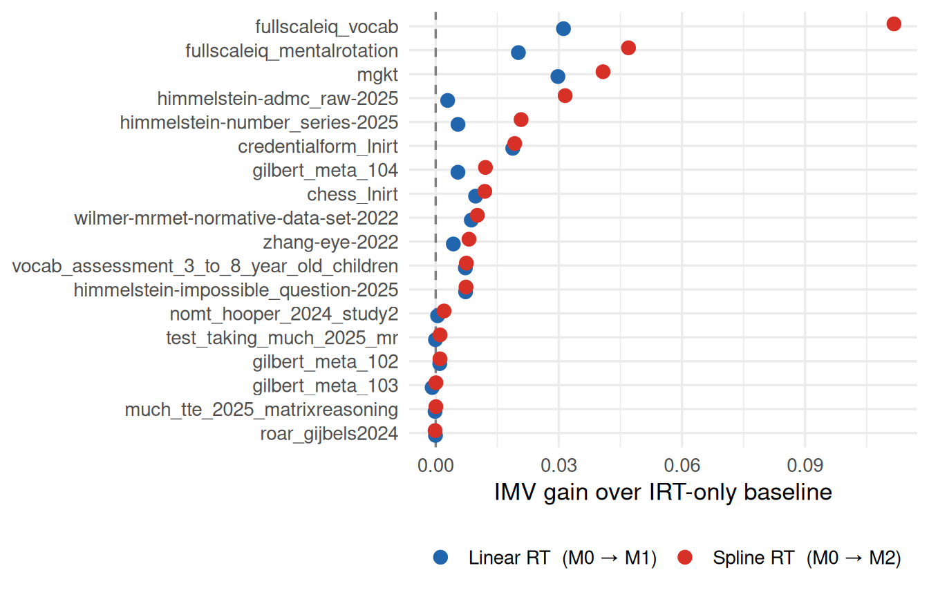
Figure 1: IMV gain from adding RT to IRT predictions. Blue = linear RT (M0→M1); red = spline RT (M0→M2). Positive values indicate RT improves predictions. Datasets ordered by spline IMV.

Across 18 datasets, the median IMV gain from adding linear RT is 0.0054 (78% of datasets positive); the spline gain is 0.0091 (94% positive).

Discussion

RT adds modest but consistent predictive value. Positive IMV for both linear and spline RT indicates that response time generally adds value in prediction of accuracy.

In some cases, the gains come from adding RT nonlinearly. RT can be a highly nonlinear predictor of response time. Indeed, the relationship between response time and accuracy may even be nonmonotonic.

Reproducibility

Results computed May 20, 2026. To regenerate:

Rscript vignettes/rt_imv_compute.R
quarto::quarto_render("vignettes/rt_imv.qmd")

References

De Boeck, Paul, Marjan Bakker, Robert Zwitser, et al. 2011. “The Estimation of Item Response Models with the Lmer Function from the Lme4 Package in R.” Journal of Statistical Software 39 (12): 1–28. https://doi.org/10.18637/jss.v039.i12.

Domingue, Benjamin W., Klint Kanopka, Ben Stenhaug, et al. 2022. “Speed–Accuracy Trade-Off? Not so Fast: Marginal Changes in Speed Have Inconsistent Relationships with Accuracy in Real Data.” Journal of Educational and Behavioral Statistics 47 (5): 576–602. https://doi.org/10.3102/10769986221099115.