| Table | m | How m is established |
|---|---|---|
| enem_2013_1mil_mt | 5 | marked letters, and ENEM 2023 item text |
| enem_2013_1mil_lc | 5 | marked letters, and ENEM 2023 item text |
| enem_2013_1mil_ch | 5 | marked letters, and ENEM 2023 item text |
| enem_2013_1mil_cn | 5 | marked letters, and ENEM 2023 item text |
| enem_2014_1mil_ch | 5 | marked letters, and ENEM 2023 item text |
| enem_2019_1mil_ch | 5 | marked letters, and ENEM 2023 item text |
| enem_2019_1mil_lc | 5 | marked letters, and ENEM 2023 item text |
| enem_2024_1mil_ch | 5 | marked letters, and ENEM 2023 item text |
| gilbert_meta_1 | 4 | item text |
| gilbert_meta_102 | 5 | item text |
| gilbert_meta_103 | 5 | item text |
Guessing in Multiple-Choice Data: Which Correction Helps Out-of-Sample?
When guessing is present in multiple-choice data, which correction actually helps out-of-sample – and when does the correction itself become a liability? Three published lenses on guessing (ability-based guessing, person-level purification, and a two-class mixture “safety valve”) plus the standard IRT baselines, compared on real IRW tables using out-of-sample IMV.
Motivation
Multiple-choice items let respondents get a question right without knowing the answer. Three literatures locate that guessing behavior in three different places, and each proposes a different fix:
- San Martín et al. (2006) locate it in a person × item interaction: the 1PL-AG model lets the probability of a correct guess itself depend on ability, via a weight \(\alpha\) on top of a per-item floor. When \(\alpha=0\) the model reduces to a fixed per-item floor (1PL-G); \(\alpha \ne 0\) means more able examinees guess more successfully – partial knowledge leaking into the “guess” itself.
- Torres Irribarra et al. (2026) locate it at the person level, in the calibration sample: rather than adding a guessing parameter to the item response function, their Method A flags examinees whose response pattern looks more like a flat guessing process than a Rasch process, removes them from calibration, and refits. No new item parameter is introduced; the item parameters themselves are what improve.
- Xiao et al. (2026) (the “Safety Valve” paper) locate it in a discrete latent class: a two-class mixture in which one class responds according to a Rasch model and the other responds at a fixed chance level, with the mixing proportion \(\pi\) estimated from the data. As \(\hat\pi \to 1\) the model collapses to a plain Rasch model, so (per their central finding) it costs almost nothing when guessing is absent, while a fixed-floor 1PLg can pay a large, asymmetric predictive penalty when its assumed floor doesn’t match the population.
None of these three papers puts all three lenses, plus the standard Rasch/2PL/1PLg/3PL baselines, on one predictive scale across a battery of real datasets. That’s the contribution here: fit all seven specifications on real IRW tables and score every one of them on genuinely held-out responses, using the InterModel Vigorish [IMV; Domingue et al. (2025)].
Explore the model shapes
Rasch and 1PLg apply the same floor to every examinee, regardless of whether they’re guessing or working the problem. 1PL-AG tilts that floor by ability. The Mixture model only applies the floor to the estimated share of guessers. Drag the sliders below to see how the five item characteristic curves (ICCs) relate to one another.
Data and methods
Data selection
Guessing corrections only make sense for genuine single-answer, multiple-choice items with a well-defined chance level – so the candidate pool needed to satisfy several requirements simultaneously: dichotomous (correct/incorrect) responses, construct_type == "Cognitive/educational" (guessing is a multiple-choice-test phenomenon, not a Likert/personality-item one), sufficient sample size for the two custom estimators below to be stable, and – critically – a verifiable, homogeneous number of response options \(m\) per table, since every model here needs a chance level \(1/m\).
A first pass required IRW item text (to count response options directly) plus construct_type/n_categories/n_participants metadata filters. That produced 26 metadata-plausible candidates, but manual inspection of the actual item text excluded most of them: some “options” columns turned out to be scoring-rubric labels (Correct/Incorrect/Self-correct) rather than response alternatives an examinee chooses from; some items were “choose two words” formats with a non-standard chance structure; one was an Agree/Disagree/Not-Sure belief inventory rather than a distractor-based knowledge test. Only three tables survived as genuine, item-text-verified, single-answer MC with a homogeneous option count: gilbert_meta_1 (m=4), gilbert_meta_102 (m=5), and gilbert_meta_103 (m=5), all from the same underlying literacy-intervention study.
That pool alone was thin and not very representative of the high-stakes settings where guessing corrections matter most. ENEM (Brazil’s national university-admissions exam) is documented as a 5-option (A-E) multiple choice test across subjects and years, and the check below confirms \(m = 5\) from the data. We use it for 8 ENEM candidate tables spanning 2013, 2014, 2019, and 2024 and all four subject areas (mt=math, lc=languages, ch=human sciences, cn=natural sciences), restricted to the density=1 table/years (every respondent answered the identical fixed item set, no rotated-booklet missingness). All eight are analysed; enem_2019_1mil_lc was excluded from an earlier version of this page on answer-key grounds that the v52.0 rebuild removed (see Screening the answer key). Note that density=1 does not mean no missingness at all: both lc tables carry the elective English/Spanish block, which every candidate answers exactly half of. Each ENEM table has roughly a million respondents; we work with a fixed-seed random subsample of 3000 per table for compute tractability.
IRW carries no item text for these eight tables, so \(m\) cannot be counted from options as it is for the gilbert_meta tables. It can be checked another way. The ENEM tables record the letter each candidate marked, and on all 370 items across the eight tables every one of A-E was chosen. Even the least-chosen letter on any item drew 1.4% of the candidates who answered it (14,111 people), which rules out a four-option item, and nothing besides A-E, a blank and a double mark occurs anywhere, which rules out a sixth option. The adjacent year does carry item text: 184 of 184 ENEM 2023 items have exactly five options, A to E, and each of the four booklets says so in its instructions (“são apresentadas 5 opções”). So \(m = 5\) here is checked, not assumed (guessing_m_check.R).
Per Xiao et al. (2026) (Section 3.2), two-alternative forced-choice (2AFC) items are excluded from this design on principle, not just by happenstance: at \(g_{\text{fit}}=0.5\) the Rasch model already predicts roughly 0.5 on sufficiently difficult items, so the Mixture model’s two classes are not empirically separable – the guessing class predicts a flat 0.5 that the engaged class already produces for low-ability respondents on hard items. All tables used here have \(m \ge 4\), safely inside the class-separated region the Safety Valve paper establishes.
Screening scored absences
One further screen runs before any model is fit. On the current data it removes almost nobody; it is on the page because, on an earlier release of these tables, it mattered more than any modelling choice here.
On a \(J\)-item, \(m\)-option test, a candidate who guesses every item scores about \(J/m\) – roughly 9 of 45 at \(m = 5\). Scoring zero on 45 answered items has probability around \(4\times10^{-5}\). So a block of candidates at or near zero is not the lower tail of ability, and it is certainly not guessing: it is absence recorded as a wrong answer. Before the ENEM rebuild in IRW dataset v52.0, five of the eight ENEM tables carried exactly such a block, at roughly 45% of the drawn sample, with almost nobody between 1 and 3 correct – a spike at zero and then a normal-looking distribution starting above the chance floor. The rebuild recodes a section the candidate did not sit as missing rather than wrong, and the block is gone.
This is the same coding artifact as the elective-block problem described in guessing_compute.R’s item-level screen – a section the candidate did not sit, scored 0 rather than left missing – but at the candidate level rather than the item level, so an item-level check cannot see it. The screen stays as a safeguard: any table with the same defect would otherwise pass straight into the fits.
Every candidate is therefore tested against the lower tail of \(\mathrm{Binomial}(J_i, 1/m)\), where \(J_i\) counts the items that candidate actually answered, and dropped when \(P(\text{score} \le \text{observed}) < 10^{-3}\). The cut is stated as a tail probability rather than a raw-score threshold so that it adapts to tables with different \(J\), different \(m\), and different per-candidate missingness. It is deliberately strict: on the rebuilt tables it removes at most a handful of candidates from each.
| Table | N analysed | N screened out | % screened |
|---|---|---|---|
| enem_2013_1mil_mt | 2998 | 2 | 0.1% |
| enem_2013_1mil_lc | 2998 | 2 | 0.1% |
| enem_2013_1mil_ch | 3000 | 0 | 0.0% |
| enem_2013_1mil_cn | 3000 | 0 | 0.0% |
| enem_2014_1mil_ch | 2997 | 3 | 0.1% |
| enem_2019_1mil_ch | 2996 | 4 | 0.1% |
| enem_2019_1mil_lc | 2996 | 4 | 0.1% |
| enem_2024_1mil_ch | 2997 | 3 | 0.1% |
| gilbert_meta_1 | 2999 | 1 | 0.0% |
| gilbert_meta_102 | 1913 | 1 | 0.1% |
| gilbert_meta_103 | 1914 | 0 | 0.0% |
Left in, those candidates did not degrade the fits gently; they changed what the models said. On the five affected tables the estimated latent SD ran 2.2 to 2.9 unscreened and 0.4 to 0.7 screened, and every item’s guessing parameter was driven to the no-guessing boundary – a floor model cannot fit observed zeros where it predicts \(\mathrm{expit}(\gamma)\), so it sends \(\gamma\) to \(-\infty\). An earlier version of this page reported the unscreened fits and read the inflated spread and the vanishing floor as two separate findings about guessing; they were one artifact seen twice. The screened estimates from that release land within noise of the ones on this page, so the screen had been recovering the right answer from the contaminated tables; what the rebuild adds is sample size, roughly 3,000 candidates per table where the screen had left about 1,660.
Screening the answer key
The scored-absence screen removes candidates. It cannot tell you whether the responses that remain were scored against the right key. On an earlier release of the ENEM tables one table failed that prior question badly enough to be excluded; on the rebuilt tables every one passes, and the table below is the evidence rather than an assurance. It also raises the one caveat that survives the rebuild.
Two statistics say so, neither of them a model fit. The first is item difficulty against the chance floor: on an \(m\)-option item scored correctly, \(p_j < 1/m\) should be uncommon, because a candidate who knows nothing still guesses right \(1/m\) of the time. The second, and the sharper one, is the item-total point-biserial — each item’s correlation with the total of the other items. A correctly keyed item correlates positively with the rest of the test whatever its difficulty; an item keyed to the wrong option correlates with it near zero.
| Table | m | J analysed | median p | % items p < 1/m | median item-rest r | % items r < 0.05 |
|---|---|---|---|---|---|---|
| enem_2013_1mil_mt | 5 | 45 | 0.23 | 42% | 0.201 | 20% |
| enem_2013_1mil_lc | 5 | 50 | 0.39 | 4% | 0.270 | 2% |
| enem_2013_1mil_ch | 5 | 45 | 0.35 | 11% | 0.225 | 4% |
| enem_2013_1mil_cn | 5 | 45 | 0.22 | 44% | 0.109 | 13% |
| enem_2014_1mil_ch | 5 | 45 | 0.40 | 20% | 0.228 | 4% |
| enem_2019_1mil_ch | 5 | 45 | 0.34 | 13% | 0.272 | 4% |
| enem_2019_1mil_lc | 5 | 50 | 0.39 | 6% | 0.320 | 8% |
| enem_2024_1mil_ch | 5 | 45 | 0.43 | 4% | 0.367 | 0% |
| gilbert_meta_1 | 4 | 30 | 0.55 | 0% | 0.494 | 3% |
| gilbert_meta_102 | 5 | 36 | 0.61 | 8% | 0.431 | 0% |
| gilbert_meta_103 | 5 | 29 | 0.46 | 0% | 0.407 | 0% |
No table fails. The median item-rest correlation runs from 0.11 to 0.49, and at most 20% of any table’s items correlate below 0.05 with the rest of the test.
enem_2019_1mil_lc was excluded from an earlier version of this page on exactly these statistics: one of its two elective language blocks came back scored zero for every candidate who sat it, and most of the remaining items correlated below 0.05 with the rest. Both were artifacts of how IRW aligned that table’s responses to items, fixed in the v52.0 rebuild. On the rebuilt table its median item-rest correlation is 0.32, against 0.11 to 0.37 on the other ENEM tables, and it is back in every comparison below.
The caveat is the chance floor itself. On enem_2013_1mil_cn and enem_2013_1mil_mt, 44% and 42% of the items sit below \(1/m\), against at most 20% on any other table, and on those items the median item-rest correlation is 0.08 and 0.16: weak, and close to zero on the first, but positive, where items keyed to the wrong option would sit at zero or below. Hard forms are the likelier explanation, though not a proven one. enem_2013_1mil_cn is the weaker of the two, with the lowest median item-rest correlation of any table here (0.11). Either way it matters for what follows. The 1PLg fixes every item’s floor at \(1/m\), the Mixture’s guessing class answers at \(1/m\), and the 3PL’s prior centres its floor near there, while these items show no such floor in the data. On these tables the fixed-floor models rest on an assumption the data do not support.
What an estimated floor of \(1/m\) looks like
The results table below reports the guessing floor the 1PL-G stage recovers, \(\mathrm{expit}(\hat\gamma_j)\), summarised over items. Reading that column requires knowing what a correct floor of \(1/m\) looks like once it has been estimated, and the answer is: not much like \(1/m\).
Two things push it around. The summary over items matters — the maximum over \(J\) items is an extreme order statistic and is biased upward by construction, which is why this page reports the median. And the floor is entangled with the latent variance: a guessing floor and a small ability spread both flatten the lower end of the item response function, so the two parameters lean on each other, and the narrower the spread the harder they are to separate. The ENEM tables sit at \(\mathrm{SD}(\theta) = 0.4\) to \(0.9\) under Rasch, which is the worst part of that range.
guessing_floor_calibration_compute.R generates from the 1PL-G with a floor of exactly \(1/m = 0.20\) on every item, at the \(N\) and \(J\) of these tables, and fits it with the same estimator the page uses:
| True SD(θ) | True floor | Recovered median floor | Recovered max floor | Recovered SD(θ) |
|---|---|---|---|---|
| 0.4 | 0.2 | 0.278 (0.216-0.337) | 0.627 (0.552-0.689) | 0.49 |
| 0.7 | 0.2 | 0.205 (0.182-0.232) | 0.419 (0.372-0.502) | 0.71 |
| 1.0 | 0.2 | 0.203 (0.191-0.213) | 0.356 (0.291-0.481) | 1.01 |
| 1.4 | 0.2 | 0.197 (0.184-0.211) | 0.286 (0.256-0.317) | 1.39 |
At a true spread of 0.4 a true floor of 0.20 comes back with a median of 0.28 and a maximum of 0.63, and the estimated spread itself runs high (0.49 against 0.4) – the floor and the variance absorb each other’s bias. By 1.4 the median is 0.20 and the maximum 0.29. Two consequences for the column below. First, the maximum is not evidence about the level of the floor in this regime, only about whether any floor survives, which is the question the identification check needs it for. Second, the observed medians (0.15 to 0.23 across the tables here) are consistent with a true floor at 1/m, but they cannot establish it: at these spreads the estimator would return numbers in that range from a floor of exactly 1/m, and the page claims no more than that.
Models fit
Seven specifications per table:
- Rasch – no guessing correction.
- 2PL –
mirt, lognormal(0,1) prior on \(a_1\) (this site’s existing convention; seeimv.qmd). - 1PLg – fixed floor \(g=1/m\), discrimination fixed at 1, difficulty free (built via a constrained 3PL in
mirt). - 3PL –
mirt, lognormal(0,1) prior on \(a_1\) (same as 2PL, chosen for internal consistency rather than replicating the Safety Valve paper’s tighter lnorm(0,0.5)) and Beta(5,17) on \(g\) (mean \(\approx 0.23\)), per the Safety Valve paper’s Study 5. - 1PL-AG (San Martín et al. 2006) – standalone marginal-likelihood estimator (
vignettes/guessing_helpers.R::fit_1pl_ag()), quadrature-integrated, with an analytic gradient verified against finite differences before use. Reports the likelihood-ratio test of \(\alpha=0\). - Mixture (“safety valve”) (Xiao et al. 2026) – standalone estimator (
fit_mixture()), multi-start over \(\pi_0 \in \{0.6, 0.75, 0.9, 0.97\}\), gradient likewise verified. - Purified Rasch (Method A) (Torres Irribarra et al. 2026) – flags examinees whose response pattern favors a flat-guessing likelihood over the Rasch likelihood, removes them, refits Rasch on the retained sample (
purify_rasch()). Its held-out predictions are evaluated on the full sample (including flagged persons), since the promise of purification is better item parameters, not that flagged persons are themselves predicted well.
All seven specifications estimate the latent variance. mirt’s itemtype = "Rasch" fixes every slope at 1 and estimates \(\mathrm{Var}(\theta)\), so the three standalone estimators (fit_1pl_ag(), fit_mixture(), purify_rasch()) do the same rather than pinning \(\theta \sim N(0,1)\). The 1PLg needs it done by hand. It is fit as a constrained mirt 3PL, and mirt frees the variance automatically only for itemtype = "Rasch"; a 3PL with its slopes pinned at 1 keeps \(\mathrm{Var}(\theta) = 1\) unless told otherwise, which leaves nothing free to set the scale. An earlier version of this page missed this. Pinned, the 1PLg ran out its 2,000-cycle budget on seven of the eleven tables, and the page reported those cells as blank for non-convergence and called the pattern unexplained. With the variance freed it converges on every table in under 50 cycles. This matters more than it sounds. If the baseline estimates a variance the Mixture does not, the two are not nested, and the Mixture cannot collapse onto Rasch as \(\hat\pi \to 1\) – which is exactly the safety-valve property this page sets out to test. On simulated data containing no guessing at all, that mismatch alone drove IMV(Rasch, Mixture) to \(-0.002\) at \(\mathrm{SD}(\theta) = 1.6\); with the variance free it stays within \(\pm 0.0002\) across the same range. The effect on the 1PL-AG’s \(\alpha\) was larger still: with the prior pinned and a true \(\mathrm{SD}(\theta)\) of 1.4, \(\hat\alpha\) came back \(-0.46\) when the truth was 0 and \(-0.42\) when the truth was \(+0.5\) – a sign flip, and a negative \(\alpha\) turns the item characteristic curve over at the low end. Freeing the variance returns \(+0.003\) and \(+0.38\) on the same data.
Before use on real data, fit_1pl_ag() and fit_mixture() were validated by simulation: both correctly return a non-significant likelihood-ratio test / \(\hat\pi \approx 1\) under a true null (no guessing), and both recover known parameters reasonably well under a true alternative (Mixture recovery was excellent; 1PL-AG’s \(\beta\) recovered well but its \(\gamma\) was noisy at moderate sample sizes – a limitation the source paper documents for its own real-data application, not an implementation defect). See Limitations below.
Cross-validation
A single 80/20 response-level (cell) holdout per table, masked once and reused across all seven model fits, per this codebase’s existing convention (Stenhaug and Domingue (2022)) – masking is per-person and always leaves at least one retained response. This is a single split, not the 20 repeated splits used in the Safety Valve paper’s own empirical section (see Limitations).
Results
All predictive comparisons below are framed relative to a single common baseline – the Rasch model, i.e. “1PL”, the no-guessing reference every other specification is trying to improve on. Rather than the scattered pairwise comparisons a first pass might reach for (1PLg vs. Mixture, 3PL vs. 1PL-AG, and so on), every model’s IMV is computed the same way, compute_imv(rasch_predictions, model_predictions, y), on the same held-out cells. That puts all six non-Rasch specifications for a table on one shared scale: positive means “beats plain Rasch out of sample,” negative means “costs something relative to just ignoring guessing entirely.”
| Table | m | N | J | N held-out | SD(θ) | π̂ (Mixture) | median expit(γ̂) (1PL-G), IQR | α̂ (1PL-AG, p) | Frac. flagged (Purified) |
|---|---|---|---|---|---|---|---|---|---|
| enem_2013_1mil_mt | 5 | 2998 | 45 | 26982 | 0.51 | 0.671 | 0.16 (0.14-0.22) | -0.098 (p=0.000) | 0.295 |
| enem_2013_1mil_lc | 5 | 2998 | 50 | 26982 | 0.71 | 0.917 | 0.19 (0.13-0.24) | 0.183 (p=0.000) | 0.171 |
| enem_2013_1mil_ch | 5 | 3000 | 45 | 27000 | 0.59 | 0.939 | 0.20 (0.14-0.28) | 0.152 (p=0.000) | 0.166 |
| enem_2013_1mil_cn | 5 | 3000 | 45 | 27000 | 0.41 | 0.880 | 0.18 (0.14-0.22) | -0.128 (p=0.000) | 0.245 |
| enem_2014_1mil_ch | 5 | 2997 | 45 | 26973 | 0.62 | 0.945 | 0.18 (0.12-0.26) | 0.072 (p=0.014) | 0.128 |
| enem_2019_1mil_ch | 5 | 2996 | 45 | 26964 | 0.69 | 0.800 | 0.17 (0.13-0.22) | -0.159 (p=0.000) | 0.248 |
| enem_2019_1mil_lc | 5 | 2996 | 50 | 26964 | 0.73 | 0.895 | 0.15 (0.10-0.21) | -0.000 (p=0.985) | 0.159 |
| enem_2024_1mil_ch | 5 | 2997 | 45 | 26973 | 0.86 | 0.838 | 0.17 (0.12-0.22) | -0.002 (p=0.947) | 0.212 |
| gilbert_meta_1 | 4 | 2999 | 30 | 17329 | 1.24 | 0.692 | 0.19 (0.14-0.22) | -0.079 (p=0.001) | 0.314 |
| gilbert_meta_102 | 5 | 1913 | 36 | 13315 | 1.19 | 0.889 | 0.18 (0.06-0.28) | 0.237 (p=0.000) | 0.147 |
| gilbert_meta_103 | 5 | 1914 | 29 | 9235 | 1.00 | 0.744 | 0.23 (0.20-0.26) | 0.051 (p=0.083) | 0.308 |
| table | 2PL | 1PLg | 3PL | 1PL-AG | Mixture | Purified Rasch |
|---|---|---|---|---|---|---|
| enem_2013_1mil_mt | 0.0107 | 0.0061 | 0.0158 | 0.0161 | 0.0065 | -0.0065 |
| enem_2013_1mil_lc | 0.0098 | 0.0048 | 0.0105 | 0.0107 | 0.0023 | -0.0019 |
| enem_2013_1mil_ch | 0.0085 | -0.0035 | 0.0106 | 0.0092 | 0.0010 | -0.0025 |
| enem_2013_1mil_cn | 0.0058 | -0.0029 | 0.0094 | 0.0086 | 0.0013 | -0.0030 |
| enem_2014_1mil_ch | 0.0088 | -0.0026 | 0.0105 | 0.0100 | 0.0015 | -0.0011 |
| enem_2019_1mil_ch | 0.0124 | 0.0064 | 0.0161 | 0.0139 | 0.0058 | -0.0036 |
| enem_2019_1mil_lc | 0.0123 | 0.0033 | 0.0139 | 0.0127 | 0.0039 | -0.0041 |
| enem_2024_1mil_ch | 0.0124 | 0.0100 | 0.0173 | 0.0141 | 0.0076 | -0.0035 |
| gilbert_meta_1 | 0.0149 | 0.0170 | 0.0205 | 0.0197 | 0.0126 | -0.0116 |
| gilbert_meta_102 | 0.0130 | 0.0050 | 0.0144 | 0.0124 | 0.0062 | -0.0039 |
| gilbert_meta_103 | 0.0157 | 0.0176 | 0.0244 | 0.0249 | 0.0072 | -0.0096 |
The table above fixes the baseline at Rasch. The widget below lets you pick any two of the seven specifications and see IMV(m1, m2) – m1 as baseline, m2 as the model being evaluated – across every table, without re-fitting anything (every pairwise value was precomputed from the same cached held-out predictions used everywhere else on this page). IMV is directional, so IMV(Rasch, 3PL) and IMV(3PL, Rasch) are not mirror images of each other – pick both orders if you want to see that asymmetry directly.
What to notice
Least guessing detected: enem_2014_1mil_ch has π̂ = 0.945 – the Mixture model assigns the largest engaged share of any table here, with IMV(Rasch,Mixture) of 0.0015.
Substantial guessing detected: enem_2013_1mil_mt has π̂ = 0.671, meaning the Mixture model assigns roughly 33% of response weight to the guessing class, with IMV(Rasch,Mixture) of 0.0065.
Does the safety valve hold?
The Mixture’s central claim is not that it wins. It is that it costs nothing when there is nothing to correct: as \(\hat\pi \to 1\) the guessing class empties out, the model collapses onto the Rasch baseline, and the analyst who fitted it anyway is no worse off. Every model on this page estimates the latent variance precisely so that this collapse is available to it (see Models fit) – with the Rasch baseline estimating a variance the Mixture did not, the two would not be nested and the collapse could not happen however far \(\hat\pi\) went.
An earlier version of this page made that argument on simulated data and on enem_2014_1mil_ch, whose apparent collapse turned out to be the zero block. Here it is on the tables as they stand after the scored-absence screen.
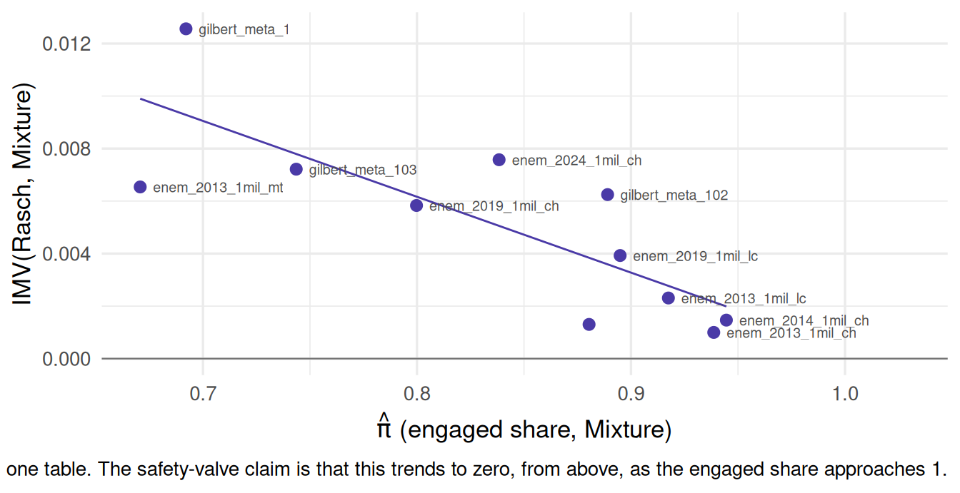
It holds, as far as 11 tables and a single split can show it, though as a tendency rather than a clean law. The Mixture’s gain over Rasch falls as the engaged share grows (r = -0.80 across tables): its largest gain, +0.0126, is on gilbert_meta_1 at \(\hat\pi\) = 0.69, while enem_2014_1mil_ch, where the guessing class is emptiest at \(\hat\pi\) = 0.94, gains +0.0015. The scatter around that is real – enem_2013_1mil_mt has the fullest guessing class of all at \(\hat\pi\) = 0.67 and still gains only +0.0065, less than gilbert_meta_1, so no single table carries the pattern. It is positive on 11 of the 11, and negative on none.
What this does not show is a table at \(\hat\pi\) close to 1. The largest engaged share here is 0.94, so the collapse is visible as a trend rather than at its endpoint, and the simulation is still what carries the endpoint. Nor does it show the valve is free in general: these are single-split margins, small enough that the sign on any one table should not be read as settled (see Limitations). The claim it supports is the modest one – across this range, fitting the Mixture where the data do not want it costs essentially nothing, which is the property the fixed-floor 1PLg conspicuously lacks (see How much does the assumed g matter?).
Two scorecards for Method A
Purified Rasch is negative in the table above on every table. Read as a leaderboard, that says the method fails. It is the wrong yardstick. Method A proposes no new item response function and makes no claim about predicting responses; it removes guessing-contaminated persons from the calibration sample so that the surviving item parameters are less distorted. Held-out response prediction is the yardstick built for models that exist to predict responses.
The check that its own logic asks for needs a known truth, so this one is a simulation (vignettes/guessing_sim_compute.R): a two-class mixture with a share \(\pi\) of engaged Rasch responders and the rest answering at a flat \(g=0.2\) on every item, with the generating difficulties \(b_{true}\) known. Both scorecards are computed on the same fitted runs – RMSE of the recovered difficulties against \(b_{true}\) (both centred, since \(b\) is identified only up to location), and held-out IMV against Rasch.
| π (true) | π̂ | Frac. flagged | RMSE Rasch | RMSE Purified | RMSE Mixture | Slope Rasch | Slope Purified | IMV Purified | IMV Mixture |
|---|---|---|---|---|---|---|---|---|---|
| 0.70 | 0.703 | 0.286 | 0.355 | 0.061 | 0.061 | 1.41 | 1.00 | -0.0108 | +0.0234 |
| 0.80 | 0.798 | 0.210 | 0.249 | 0.058 | 0.056 | 1.25 | 0.99 | -0.0051 | +0.0172 |
| 0.90 | 0.900 | 0.126 | 0.135 | 0.058 | 0.053 | 1.11 | 0.98 | -0.0016 | +0.0091 |
| 1.00 | 1.000 | 0.047 | 0.048 | 0.059 | 0.048 | 1.00 | 0.98 | -0.0000 | +0.0001 |
With 20% of respondents replaced by flat guessers, Rasch recovers difficulty with RMSE 0.249 and Purified Rasch with 0.058 – purification is 4.3 times more accurate on the parameters – while giving up 0.0051 in IMV on the very same fitted runs. Rasch’s recovery slope of 1.25 is the mechanism: guessing compresses a Rasch calibration toward the middle, and purification (slope 0.99) largely undoes that.
So the negative column is what this method looks like when it is working, not evidence against it. Two scorecards, different winners.
Method A has no safety valve of its own, though. On the no-guessing row it still flags 4.7% of respondents and drops them from calibration, and recovery gets slightly worse than plain Rasch as a result (RMSE 0.059 vs. 0.048). The cost is small, but unlike the Mixture – which collapses onto its Rasch baseline when there is nothing to correct – purification always pays something for the persons it removes.
One caveat on reading this as a defence of Method A specifically: the Mixture model wins both scorecards here (RMSE 0.056, IMV +0.0172). The data-generating process is the Mixture’s own assumed model, so this is its home turf and the comparison is not a fair horse race between the two corrections. The point is narrower – that the sign of Purified Rasch’s IMV column carries no information about whether purification did its job.
How much does the assumed \(g\) matter?
Every fixed-\(g\) model above is handed \(g = 1/m\), so the analyst is right by construction on every table on this page. That is the one axis the main run does not vary, and it is the axis Xiao et al. (2026)’s Studies 1 and 3 are built on. vignettes/guessing_gsweep_compute.R refits the 1PLg and the Mixture across a grid of assumed \(g\) values on each real table, scoring both against a common Rasch baseline on the same holdout convention.
The two models mis-specify differently. The 1PLg pushes every person’s floor to the assumed \(g\), so a wrong \(g\) is wrong for every response. The Mixture applies \(g\) only to the share of response weight it assigns to the guessing class, and can shrink that share when \(g\) fits badly – the safety valve. The prediction is that the 1PLg should be far more sensitive.
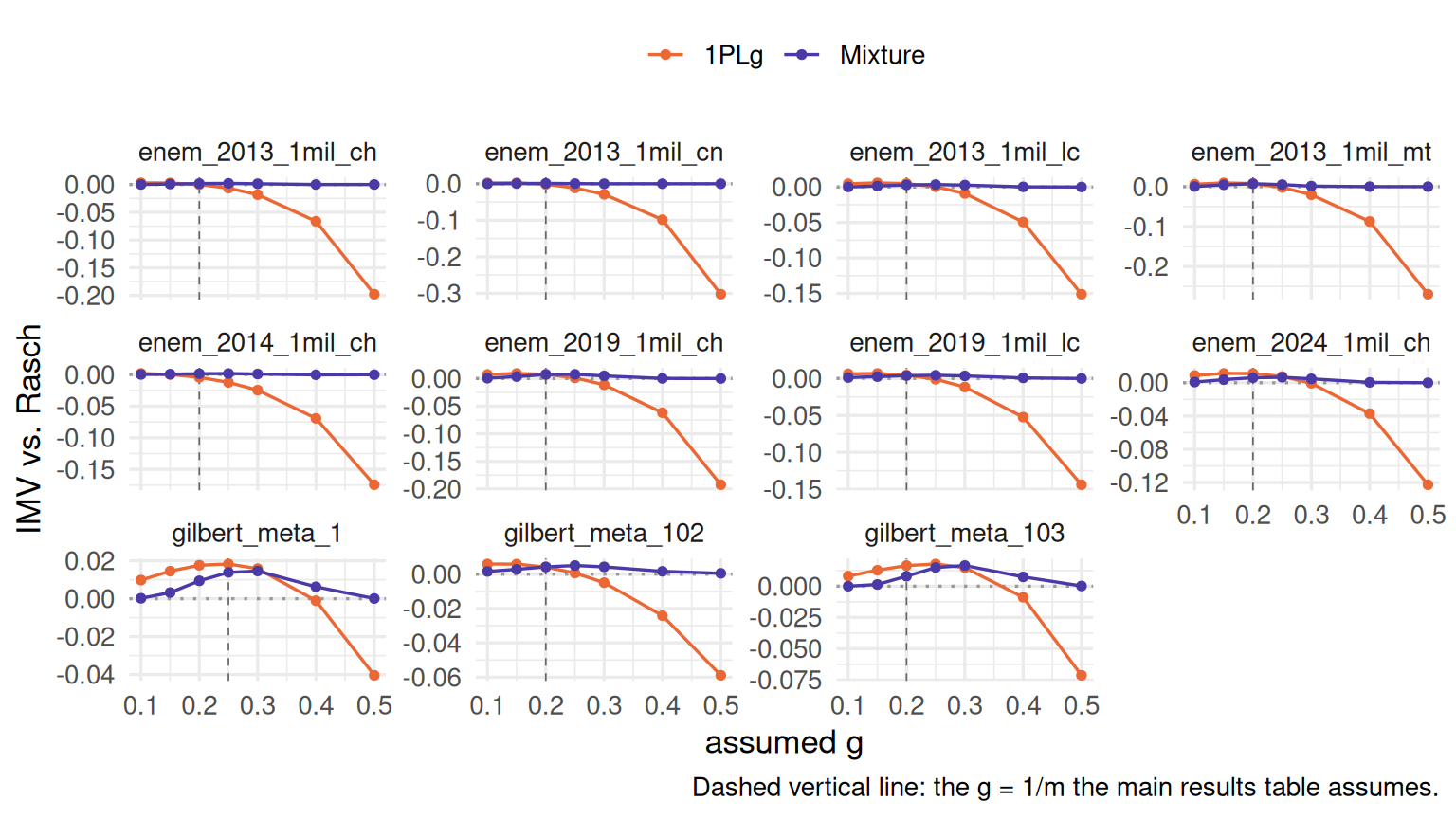
Across the 11 tables, moving the assumed \(g\) over the range [0.10, 0.50] moves the 1PLg’s IMV by a median of 0.157 (worst table 0.305) and the Mixture’s by a median of 0.005 (worst 0.017). The worst single 1PLg value anywhere on the grid is -0.302, against -0.0004 for the Mixture. The asymmetry is the practical content of the safety-valve claim: a fixed-floor model is only as good as the analyst’s \(g\), whereas the Mixture degrades toward its Rasch baseline instead of past it.
Those two worst-case figures come from different tables, though, so the gap between them overstates the asymmetry. The Mixture’s worst table is gilbert_meta_103, and on that table the 1PLg moves 0.089 against the Mixture’s 0.017 – a ratio of 5.4, not the 34 the median-to-median comparison gives. That is the number to read: on gilbert_meta_103 the Mixture’s sensitivity to the assumed \(g\) (0.0165) is larger than the largest IMV the Mixture achieves against Rasch anywhere on this page (0.0126), and larger still than its own IMV on that table (0.0072). Where the valve matters most, it moves further with the analyst’s assumption than its entire signal.
Limitations
- The scored-absence screen is a safeguard, not a repair. On the current release of these tables it removes a handful of candidates at most (see Screening scored absences). On an earlier release it removed roughly 45% of five tables, a non-random block of candidates who had not sat the section, and the fix that mattered was upstream: IRW now records a section a candidate never took as missing, so everyone who pulls these tables gets that, not only readers of this page. A table with the same defect would still pass the screen’s results through as a range-restricted sample, which is a different estimand from the one the full candidate pool would give. That upstream fix covers whole sections only: an item left blank (
.) or double-marked (*) on a section the candidate did sit is still scored wrong rather than missing – INEP’s own scoring, on 0.43% of cells across these eight tables (0.28% blank, 0.15% double mark). Both codes survive inresp_raw, so an analysis that wants them treated as missing can recode them itself. - The level of the recovered guessing floor is not pinned down. At the sample sizes and latent spreads of these tables, a floor of exactly \(1/m\) is recovered high and with wide item-to-item scatter, and the estimated latent SD is biased in the same direction at the same time (see What an estimated floor of \(1/m\) looks like). The floor column supports “there is a floor here, and it is of a plausible size”; it does not support a comparison between a table’s floor and \(1/m\), or between one table’s floor and another’s at different spreads.
- Two tables show no floor at \(1/m\).
enem_2013_1mil_cnandenem_2013_1mil_mtput about two-fifths of their items below the chance floor (see Screening the answer key). Hard forms are the likelier reading than a key failure, thoughenem_2013_1mil_cnalso has the weakest item-rest correlations of any table on the page. Every model here that fixes or centres a floor at \(1/m\) is assuming something these two tables do not show, and their results deserve that discount. - 1PL-AG’s \(\gamma\) (and, to a lesser extent, \(\alpha\)) can be noisy. Simulation validation recovered \(\beta\) well but \(\gamma\) poorly at moderate sample sizes – consistent with San Martín et al. (2006)’s own real-data application, where some items had standard errors above 100. Point estimates of \(\hat\alpha\) should be read alongside its LR test, not in isolation.
- \(\alpha\) is not identified when the data carry no guessing floor, and the LR test cannot detect this. Where every \(\hat\gamma_j\) goes to the no-guessing boundary the likelihood is flat in \(\alpha\) – \(\alpha\) enters only through the guessing branch, \(\partial P/\partial\alpha \propto (1-r)\,s(1-s)\,\theta\) with \(s = \mathrm{expit}(\alpha\theta+\gamma)\), and a vanishing \(s\) zeroes it – so the fit returns its starting value and the test returns \(p \approx 1\), numerically indistinguishable from a genuine null. On the current tables \(\alpha\) is identified everywhere and the page flags any table where it is not. On an earlier release of the ENEM tables, before the scored-absence block was removed, five of them failed exactly this way: refitting from \(\alpha \in \{\pm 0.1, \pm 0.3\}\) returned the starting value with the log-likelihood unchanged. The general lesson is that a non-significant \(\alpha\) in a 1PL-AG fit should never be read as evidence against ability-dependent guessing without first checking that \(\hat\gamma\) is interior. The simulation validation on this page did not catch it because data generated from the 1PL-AG always has a floor by construction; it takes real data that rejects a floor to produce the failure. The argument for it here is that derivative and those refits, not a published result: the identification literature for this family runs the other way. San Martín et al. (2013) identify the 1PL-G’s item parameters and scale by fixing one item’s guessing parameter at zero — a restriction imposed to buy identification, not a boundary the data arrive at on their own, and the simultaneous collapse of every \(\gamma_j\) is not a case they treat. Park et al. (2015) carry the 1PL-G identification result over to the 1PL-AG and leave explicitly open whether it implies any practical limitation for that model; they report neither a flat likelihood nor a vanishing floor. Fariña et al. (2019) is the nearest treatment of the 1PL-G collapsing onto its nested Rasch model. Read those as evidence that this model class is fragile, and this particular failure as sitting outside what they cover.
- The recovery result is a simulation, on the Mixture’s own DGM. The two-scorecards section generates data from exactly the two-class mixture the Mixture model assumes. That is the right shape for isolating what purification does to item parameters, but it is not a neutral arena for ranking the corrections against each other, and it says nothing about how Method A behaves when guessing is ability-dependent rather than flat.
- Single 80/20 split, not repeated cross-validation. IMV estimates here reflect one holdout draw per table; they are not averaged over multiple splits the way the Safety Valve paper’s own empirical section is.
- The secondary (
gilbert_meta_*) tables come from one study family. All three item-text-verified tables share an underlying literacy-intervention study; they are not independent evidence of generalizability beyond that context. - Purified Rasch (Method A) assumes person-level, not item-level, guessing – an examinee is modeled as either guessing on everything or nothing, per Torres Irribarra et al. (2026)’s own stated simplification relative to the (person × item) process that actually generates guessing.
Reproducibility
Results were computed on September 19, 2026. To regenerate:
# 1. Fit all 7 specifications across all tables (from the project root)
source("vignettes/guessing_compute.R")

# 2. Method A parameter recovery vs. held-out IMV (simulation; no Redivis
#    access needed)
source("vignettes/guessing_sim_compute.R")

# 3. Sensitivity of the fixed-g models to the assumed guessing level
source("vignettes/guessing_gsweep_compute.R")

# 4. Answer-key diagnostics: item difficulty against the chance floor and
#    item-total point-biserials (seconds; reads the cached response matrices)
source("vignettes/guessing_key_diagnostics.R")

# 5. What an estimated guessing floor of 1/m looks like at these N, J and
#    latent spreads (simulation; no Redivis access needed)
source("vignettes/guessing_floor_calibration_compute.R")

# 6. Whether m = 5 holds for the ENEM tables: letters marked per item, and
#    the ENEM 2023 item text (server-side counts; needs REDIVIS_API_TOKEN)
source("vignettes/guessing_m_check.R")

# 7. The same pipeline on ordinary IRW cognitive tables, and the 3PL's
#    sensitivity to its prior on g (needs REDIVIS_API_TOKEN)
source("vignettes/guessing_imv_benchmark.R")

# 8. Re-render this page
quarto::quarto_render("vignettes/guessing.qmd")
Steps 2-7 write their own caches (guessingdata/guessing_sim_results.rds, guessingdata/guessing_gsweep_results.rds, guessingdata/guessing_key_diagnostics.rds, guessingdata/guessing_floor_calibration.rds, guessingdata/guessing_m_check.rds, guessingdata/guessing_imv_benchmark.rds); the page renders without them, with those sections showing a placeholder instead. The estimators themselves, and the checks behind the variance and gradient claims in Data and methods, are in vignettes/guessing_helpers.R and vignettes/guessing_vignette_checks.R.
Source code for this page: guessing.qmd · guessing_compute.R · guessing_floor_calibration_compute.R · guessing_g_sweep.R · guessing_gsweep_compute.R · guessing_helpers.R · guessing_imv_benchmark.R · guessing_key_diagnostics.R · guessing_m_check.R · guessing_sim_compute.R · guessing_vignette_checks.R
These results were computed against approximately IRW v385 (the corpus as of September 19, 2026).
Acknowledgments
We thank Xingyao Xiao and David Torres Irribarra, whose reviews of earlier versions of this page caught several errors and shaped much of its analysis. Both are authors of methods compared here (the Mixture and Method A, respectively). Errors that remain are ours.
References
Domingue, Benjamin W., Klint Kanopka, Radhika Kapoor, et al. 2024. “The InterModel Vigorish as a Lens for Understanding (and Quantifying) the Value of Item Response Models for Dichotomously Coded Items.” Psychometrika 89 (3): 1034–54. https://doi.org/10.1007/s11336-024-09977-2.
Domingue, Benjamin W., Charles Rahal, Jessica Faul, et al. 2025. “The InterModel Vigorish (IMV) as a Flexible and Portable Approach for Quantifying Predictive Accuracy with Binary Outcomes.” PLOS ONE 20 (3): e0316491.
Fariña, Pamela, Jorge González, and Ernesto San Martín. 2019. “The Use of an Identifiability-Based Strategy for the Interpretation of Parameters in the 1PL-g and Rasch Models.” Psychometrika 84 (2): 511–28.
Park, Ryoungsun, Keenan A. Pituch, JoonHo Kim, Barbara G. Dodd, and Hyewon Chung. 2015. “Marginalized Maximum Likelihood Estimation for the 1PL-AG IRT Model.” Applied Psychological Measurement 39 (6): 448–64.
San Martín, Ernesto, Guido Del Pino, and Paul De Boeck. 2006. “IRT Models for Ability-Based Guessing.” Applied Psychological Measurement 30 (3): 183–203. https://doi.org/10.1177/0146621605282773.
San Martín, Ernesto, Jean-Marie Rolin, and Luis M. Castro. 2013. “Identification of the 1PL Model with Guessing Parameter: Parametric and Semi-Parametric Results.” Psychometrika 78 (2): 341–79. https://doi.org/10.1007/s11336-013-9322-8.
Stenhaug, Ben A., and Benjamin W. Domingue. 2022. “Predictive Fit Metrics for Item Response Models.” Applied Psychological Measurement 46 (2): 136–55.
Torres Irribarra, David, Camila Echeverría, and Pablo Espinoza. 2026. Improving Item Parameter Recovery Under Guessing: A Classification Approach in High-Stakes University Admissions Tests. Symposium: Psychometric Innovations for Fairer Decisions in Chile’s National University Admissions System. Presented at ITC 2026, Auckland, NZ.
Xiao, Xingyao, Esther Ulitzsch, Lijin Zhang, Michael C. Frank, and Benjamin W. Domingue. 2026. The Safety Valve: A Mixture IRT Approach to Modeling Guessing Behavior.