Experience-sampling responses pile up at the bottom of the scale, and a recent preprint argues that ignoring that pile biases the person-level correlations that dynamic structural equation models are fitted to estimate. Its remedy is a censored model. But censoring is only one theory of what a floor is — an appropriate link models the boundedness directly, and a graded model says the floor was never special to begin with. This vignette measures how much floor mass IRW’s intensive longitudinal datasets actually carry, shows that the composite scores the field models hide almost all of it, and puts the competing models against each other on a study that randomised its participants to a Likert or a slider version of the same protocol.
Published
September 21, 2026
NotePartial run
Floor profiles: 26 of 26 curated ESM tables — complete. Model comparison: 12 of 12 fits (2 items x 2 arms x the families admissible for each). Sections below compute only from fits that are present, so a cell absent from a table has not been run rather than been excluded. Sampler settings are draft-grade; intervals will narrow in a final run.
This vignette was drafted by Claude with human review. The scoping decisions — which datasets qualify as experience sampling, and which models are being compared — came out of a written brief circulated to IRW collaborators, and the model set below was revised in response to their comments.
Motivation
Ask people how they feel several times a day for a fortnight and a lot of their answers land on the bottom of the scale. Not anxious. Not stressed. Not at all. That pile is a nuisance for the models the field fits to such data: dynamic structural equation models (DSEM) treat each person’s series as a continuous process with a mean, an autoregression, and an innovation variance, and then estimate how those person-level quantities correlate.
A recent preprint — Beneath the Floor: Censored DSEM Models for Analyzing ESM Data with Floor Effects(Beneath the Floor 2026) — argues that ignoring the pile biases exactly those correlations, most sharply the one between a person’s mean level and their innovation variance, and recommends modelling the censoring explicitly.
That recommendation carries an assumption worth naming. A censored model says there is a latent continuum extending below the boundary that we simply cannot observe — the person is somewhere below “not at all anxious”, and the scale truncated them. That is a specific and contestable claim about what a floor is, and it is not the only one available:
Censoring. A continuum runs past the boundary; the floor is truncation. Someone at the floor could have been lower.
Zero-inflation. Sitting at the floor is a different kind of event from sitting just above it. “Not at all” is a state, not a smaller amount of something. Under an inflated beta model the boundary gets its own probability and the interior gets a bounded continuous density.
Graded response. The answer was categorical the whole time. The floor is the bottom category, and nothing about it needs special handling.
These are not three ways of patching the same nuisance. They are three theories of the data, they imply different generative stories, and — usefully — they make different predictions about the very correlation the preprint reports.
IRW is a reasonable place to adjudicate because it holds intensive longitudinal data in both ordinal and near-continuous response formats, in one schema. The two vignettes closest to this one are Bounded Continuous Responses, which compares bounded-response model families cross-sectionally, and Dimensionality Across IRW, which is the template for an assumption audit run across many tables at once. This page is the time-domain sibling of the first.
That earlier vignette also left this exact question open. It stress-tested four bounded-response specifications against 20% boundary inflation and concluded that all of them degrade, because none of them includes a zero-one-inflated component — “a true zero-one-inflated extension would be needed for that” (Molenaar et al. 2022). It named the missing model and stopped. This page fits it.
Data and methods
Finding the datasets at all
IRW has no reliable handle for intensive longitudinal data, which is the first finding and the reason the pool below had to be built by hand.
metadata$longitudinal flags 703 tables, but it is a text search for wave or date in the column list, so it matches cov_birthdate and cov_startdate.
The intensive_longitudinal collection requires dateandwave together. Of its 81 members, 72 are one COVID panel study at about 2.6 waves per person, and exactly one is experience sampling. Its own definition says as much.
There is no temporal tag. The tag vocabulary covers age, sample, construct, tool, format and language — nothing about design over time.
Across 4,238 tables, 551 carry wave and 224 carry date, but only 81 carry both, so requiring both excludes most genuine ESM studies while admitting a large panel study.
What works is occasions per person — responses per participant divided by item count — followed by reading each surviving table’s processing script. That screen produced the pool used here.
Code
if (nrow(floor_summary) >0) { floor_summary |>mutate(`occ/person`=round(n_responses / n_persons / n_items, 1)) |>select(Table = table, Format = format, Persons = n_persons, Items = n_items,`occ/person`, `Time index`= occasion_col) |>arrange(desc(`occ/person`)) |>kable(caption ="The curated ESM pool, ordered by occasions per person.")}
Table 1: The curated ESM pool, ordered by occasions per person.
Table
Format
Persons
Items
occ/person
Time index
westhoff2023_pbat
Slider / continuous
113
18
96.8
wave
westhoff2023_stopd
Slider / continuous
113
5
96.8
wave
smoking_perseverance_mcneish_2025
Ordinal
50
3
70.5
date
mhscdc_fried_2020_ema
Ordinal
79
18
49.9
wave
kuehner_2017_mw_rumination
Ordinal
43
2
45.7
wave
steinberg_2023_mentalizing_momentary
Ordinal
20
3
36.9
wave
vollbracht_et_al_2026_ambulatory_assessment
Slider / continuous
406
15
36.8
trial_occasion
evpromisi_stone_2021_ddpainin
Ordinal
200
6
26.3
wave
evpromisi_stone_2021_ddeddep
Ordinal
283
8
26.2
wave
nas_rogoza_2024_study5_nas
Slider / continuous
317
4
25.9
wave
nas_rogoza_2024_study5_ngs
Slider / continuous
317
4
25.9
wave
nas_rogoza_2024_study5_nvs
Slider / continuous
317
4
25.9
wave
evpromisi_stone_2021_ddedanx
Ordinal
183
7
25.8
wave
zhang_2020_trait_creativity_mood
Slider / continuous
54
12
24.4
wave
strohacker_2024_arms_readiness
Ordinal
22
10
23.6
wave
strohacker_2024_bmzi_motive
Ordinal
22
11
23.6
wave
gilbert_meta_101
Ordinal
256
9
21.5
wave
soderberg_2024_esm_affect
Ordinal
300
8
14.6
wave
sondell_2018_dementia_motivation
Ordinal
184
2
14.4
wave
soderberg_2024_esm_lecture
Ordinal
300
6
13.9
wave
schafer_2016_music_goals
Ordinal
121
3
12.4
wave
schafer_2016_music_effects
Ordinal
121
3
12.4
wave
opentsstvr_linnig_2025_vas
Slider / continuous
98
7
10.4
wave
soderberg_2024_esm_morning
Ordinal
290
2
7.2
wave
debacker_2018_justice_appraisal
Ordinal
96
12
7.0
wave
debacker_2018_decisionjustification
Ordinal
96
4
7.0
wave
Confirming each table by script mattered: four candidates that pass any column-based screen fail on inspection. narcissism_schneider_2025_study2_* (18 tables) falls back to a survey disposition code as id, so id is not a person and the recorded participant count is 3. moralvignettes_rakhmankulova_2025 has id as a video and rater as the person. political_psychology drops wave in processing. And about 21 cognitive trial-level tasks have many measurements per person, but those are trials, not occasions.
Two more were caught only after they had been profiled, which is worth recording because it shows what the screen alone cannot do. emoji_scheffler_2024 (id is the emoji, rater the person) and tears (id is a video, rater the person) are stimulus-rating studies: many responses per id, no time dimension at all. They scored well on occasions-per-person precisely because many raters judged each stimulus. Both were dropped.
The floor is an item-level property
The field reports floor rates for a composite — the mean of the items administered at each beep. Because items within one instrument sit at very different points on the scale, that average can drive the composite’s floor mass to almost nothing while individual items remain heavily piled.
It does, and by a lot. The gap is not uniform, though, and the pattern is informative: compositing hides the floor precisely when the items disagree about where the floor is. Where every item in an instrument is heavily floored, the composite stays floored and nothing is concealed. Where one item floors and its neighbours do not, the average washes it out entirely.
Code
if (nrow(floor_summary) >0) { p <- floor_summary |>filter(!is.na(composite_floor)) |>mutate(text =sprintf("%s\nitems: %.1f%%–%.1f%% at floor\ncomposite: %.3f%%", table, floor_min, floor_max, composite_floor)) |>ggplot(aes(x = floor_max, y = composite_floor, colour = format, text = text)) +geom_abline(slope =1, intercept =0, linetype ="dashed", colour = irw_grey) +geom_point(size =2.6, alpha = .85) +scale_colour_manual(values =c("Ordinal"= irw_amber,"Slider / continuous"= irw_blue), name =NULL) +labs(x ="Highest per-item floor mass in the table (%)",y ="Floor mass of the composite (%)",title ="Averaging items hides the floor",subtitle ="Points below the dashed line: the composite understates its own worst item") +theme(legend.position ="top")ggplotly(p, tooltip ="text")}
Figure 1
In 19 of 25 tables the composite’s floor mass is less than half that of the table’s most-floored item. In 8 of them the composite sits below 1% while an item is above 20%. The extreme case is vollbracht_et_al_2026_ambulatory_assessment, where an item at 32.6% floor becomes a composite at 0.005% — a factor of roughly 7,093.
Code
if (nrow(floor_summary) >0) { floor_summary |>filter(!is.na(composite_floor)) |>mutate(hiding = floor_max - composite_floor) |>arrange(desc(hiding)) |>transmute(Table = table, Format = format,`Worst item (%)`=round(floor_max, 1),`Median item (%)`=round(floor_median, 1),`Composite (%)`=round(composite_floor, 3),`Hidden (pp)`=round(hiding, 1)) |>head(12) |>kable(caption ="Where compositing conceals the most floor mass.")}
Table 2: Where compositing conceals the most floor mass.
Table
Format
Worst item (%)
Median item (%)
Composite (%)
Hidden (pp)
mhscdc_fried_2020_ema
Ordinal
77.7
48.6
0.051
77.7
gilbert_meta_101
Ordinal
83.3
56.0
12.144
71.2
strohacker_2024_bmzi_motive
Ordinal
61.1
17.9
0.193
60.9
westhoff2023_stopd
Slider / continuous
62.7
45.7
15.037
47.6
schafer_2016_music_effects
Ordinal
50.5
23.3
6.125
44.4
soderberg_2024_esm_affect
Ordinal
44.8
22.6
0.500
44.3
westhoff2023_pbat
Slider / continuous
44.3
10.2
0.009
44.3
schafer_2016_music_goals
Ordinal
51.1
27.8
7.790
43.3
evpromisi_stone_2021_ddeddep
Ordinal
79.7
72.1
39.568
40.1
kuehner_2017_mw_rumination
Ordinal
56.8
41.6
20.265
36.5
opentsstvr_linnig_2025_vas
Slider / continuous
36.3
19.0
0.146
36.2
vollbracht_et_al_2026_ambulatory_assessment
Slider / continuous
32.6
0.4
0.005
32.6
Code
if (nrow(floor_summary) >0) { p <- floor_summary |>filter(!is.na(composite_floor)) |>mutate(spread = floor_max - floor_min,ratio = floor_max /pmax(composite_floor, .001),text =sprintf("%s\nitem floor spread: %.1f pp\nworst item %.1f%% -> composite %.3f%%", table, spread, floor_max, composite_floor)) |>ggplot(aes(x = spread, y = ratio, colour = format, text = text)) +geom_point(size =2.6, alpha = .85) +scale_y_log10() +scale_colour_manual(values =c("Ordinal"= irw_amber,"Slider / continuous"= irw_blue), name =NULL) +labs(x ="Spread of per-item floor mass within the table (percentage points)",y ="Worst item floor / composite floor (log scale)",title ="Compositing hides the floor when items disagree about where it is",subtitle ="Instruments whose items all floor together conceal nothing") +theme(legend.position ="top")ggplotly(p, tooltip ="text")}
Figure 2
sondell_2018_dementia_motivation is absent from the composite comparisons for a different and more interesting reason: it has a perfectly good wave, but across all 5,312 person-occasions only ever one item is answered at a time. Its two items were never co-administered, so there is no occasion at which a composite could be formed. It stays in the per-item figures.
The model comparison, and why it runs on this table
vollbracht_et_al_2026_ambulatory_assessment(Vollbracht et al. 2026) randomised 406 participants to complete the same ambulatory protocol with either a Likert or a slider response format, then measured them roughly 37 times each.
One correction to how this was originally scoped: the format is a between-person randomisation, not a within-person crossing. Every one of the 406 participants has exactly one cov_group value — 200 in the Likert arm, 206 in the slider arm. That is weaker than a crossed design for isolating format, but it is still a randomised manipulation of response format holding the protocol, the items and the sampling schedule fixed, which is rare.
The table also supplies a control that nobody designed. The stress item was never sliderised — it is a 1–5 item in both arms. So it functions as a within-study placebo: whatever changes for the items whose format actually changed, but not for stress, is attributable to format rather than to the people in each arm.
Code
if (nrow(item_detail) >0) { v <- item_detail |>filter(table =="vollbracht_et_al_2026_ambulatory_assessment")if (nrow(v) >0) { v |>transmute(Item = item, `Scale low`= lo, `Scale high`= hi,Categories = n_cat, `At floor (%)`=round(floor_pct, 1),`At ceiling (%)`=round(ceil_pct, 1)) |>arrange(desc(`At floor (%)`)) |>kable(caption ="Per-item floor mass in vollbracht, pooled across arms.") }}
Table 3: Per-item floor mass in vollbracht, pooled across arms.
Item
Scale low
Scale high
Categories
At floor (%)
At ceiling (%)
stress
1
5
5
32.6
3.2
att1
0
100
101
3.9
1.4
att3
0
100
101
3.4
1.3
att2
0
100
101
2.5
1.9
wt1
-50
50
101
1.0
2.3
ct1
-50
50
101
0.6
3.0
pum3
-50
50
101
0.5
3.1
cla3
0
100
101
0.4
8.0
wt2
-50
50
101
0.4
3.0
cla1
0
100
100
0.3
7.9
cla2
0
100
101
0.3
8.3
ct2
-50
50
101
0.3
4.5
pum4
-50
50
101
0.3
4.6
pum1
-50
50
101
0.2
3.9
pum2
-50
50
101
0.2
5.0
Every model uses the same mean structure and differs only in the response distribution. Carryover is written the way DSEM actually formulates it — each occasion regressed on the previous one, \(y_{it} = \mu_i + \phi(y_{i,t-1} - \mu_i) + e_{it}\) — rather than as a residual autocorrelation structure. That choice was forced by the data and is described in Limitations, but it is also the more faithful one, and it makes \(\phi\) an ordinary regression coefficient that means the same thing in all four families.
Each model then adds a person-level dispersion random effect correlated with the person intercept, because the mean-level-to-innovation-variance correlation is the parameter the preprint reports as biased.
Code
# lag_c is the previous occasion's response, centred on the person's own mean.# Shared across families; only the response distribution changes.brms::bf(resp_z ~1+ lag_c + (1| p | id), sigma ~1+ (1| p | id)) # gaussian, and censoredbrms::bf(resp_z |cens(cens_ind) ~ ..., sigma ~ ...) # floor = left-censoredbrms::bf(resp01 ~ ..., phi ~ ...) # zero-one-inflated betabrms::bf(resp_ord ~ ..., disc ~ ...) # cumulative (graded)
Which families are even admissible depends on the format, and that is part of the finding rather than an inconvenience. A zero-one-inflated beta cannot be fitted to a five-category item; a graded model is impractical on a 101-point slider. So “apply the censoring fix to both formats” — the field’s current habit — is not a choice between equally available options. For much of this data the alternatives are ruled out before anyone compares fit.
Results
How much floor mass is actually out there
Code
if (nrow(item_detail) >0) { ord <- floor_summary |>arrange(floor_max) |>pull(table) p <- item_detail |>left_join(select(floor_summary, table, format), by ="table") |>mutate(table =factor(table, levels = ord),text =sprintf("%s\nitem %s: %.1f%% at floor\nscale %g–%g (%d categories)", table, item, floor_pct, lo, hi, n_cat)) |>ggplot(aes(x = floor_pct, y = table, colour = format, text = text)) +geom_point(alpha = .7, size =1.9) +scale_colour_manual(values =c("Ordinal"= irw_amber,"Slider / continuous"= irw_blue), name =NULL) +labs(x ="Responses at the item's observed minimum (%)", y =NULL,title ="Per-item floor mass within each ESM table") +theme(legend.position ="top", axis.text.y =element_text(size =8))ggplotly(p, tooltip ="text")}
Figure 3
Two things to read off this, one of them not what we expected.
Floor mass varies enormously within a single instrument, so a table-level summary is close to meaningless — which is the case for treating the floor as an item property throughout.
The second is that the two response formats carry about the same amount of it. Going continuous does not empty the bottom of the scale in practice; a slider simply relocates where people pile up. That undercuts a tempting shortcut — “use a VAS and the problem goes away” — and it is why the model comparison below has to be run in both formats rather than only in the ordinal one.
Does the model you choose change the answer?
Code
if (nrow(stage_b) >0&&"phi_ar1"%in%names(stage_b)) {# Deliberately NOT filtered on a non-missing estimate: a fit that timed out has# no estimates, and dropping it would erase the outcome the status column# exists to report. stage_b |>transmute(Item = item, Arm = arm, Model = family,`Floor (%)`=round(floor_pct, 1),Carryover =ifelse(is.na(phi_ar1), "—",sprintf("%.3f [%.3f, %.3f]", phi_ar1, phi_ar1_lo, phi_ar1_hi)),`cor(mean, disp)`=ifelse(is.na(cor_mean_disp), "—",sprintf("%.3f", cor_mean_disp)),Rhat =ifelse(is.na(rhat_ar), "—", sprintf("%.3f", rhat_ar)),ESS =ifelse(is.na(ess_ar), "—", sprintf("%.0f", ess_ar)),`Div.`=ifelse(is.na(n_divergent), "—", sprintf("%.0f", n_divergent)),`Min`=round(mins),Sampler = status) |>arrange(Item, Arm, Model) |>kable(caption ="Same data, competing theories of the floor. The carryover coefficient is comparable across families; the correlation is not strictly so — see Limitations. Rows marked no in the OK column failed the mixing screen and are not estimates.")}
Table 4: Same data, competing theories of the floor. The carryover coefficient is comparable across families; the correlation is not strictly so — see Limitations. Rows marked no in the OK column failed the mixing screen and are not estimates.
Item
Arm
Model
Floor (%)
Carryover
cor(mean, disp)
Rhat
ESS
Div.
Min
Sampler
att1
Likert
censored
21.5
-0.169 [-0.418, 0.100]
0.312
2.866
2
0
96
did not mix
att1
Likert
cumulative
21.5
0.158 [0.008, 0.386]
0.260
1.003
747
0
20
ok
att1
Likert
gaussian
21.5
0.059 [0.010, 0.109]
-0.145
1.001
2038
41
6
ok
att1
Slider
censored
7.9
0.139 [0.088, 0.191]
-0.290
1.001
1698
0
4
ok
att1
Slider
gaussian
7.9
0.134 [0.088, 0.182]
0.090
1.001
2203
0
4
ok
att1
Slider
zoib
7.9
0.119 [0.065, 0.171]
0.027
1.000
2679
0
9
ok
stress
Likert
censored
29.6
-0.336 [-0.894, 0.259]
-0.662
2.235
3
0
110
did not mix
stress
Likert
cumulative
29.6
0.415 [0.150, 0.795]
0.418
1.009
260
0
121
under-sampled
stress
Likert
gaussian
29.6
0.189 [0.157, 0.221]
0.179
1.001
3545
0
6
ok
stress
Slider
censored
40.0
0.168 [0.060, 0.314]
-0.810
2.128
3
0
35
did not mix
stress
Slider
cumulative
40.0
0.381 [0.150, 0.711]
0.473
1.013
199
0
32
did not mix
stress
Slider
gaussian
40.0
—
—
—
—
—
45
timed out
Code
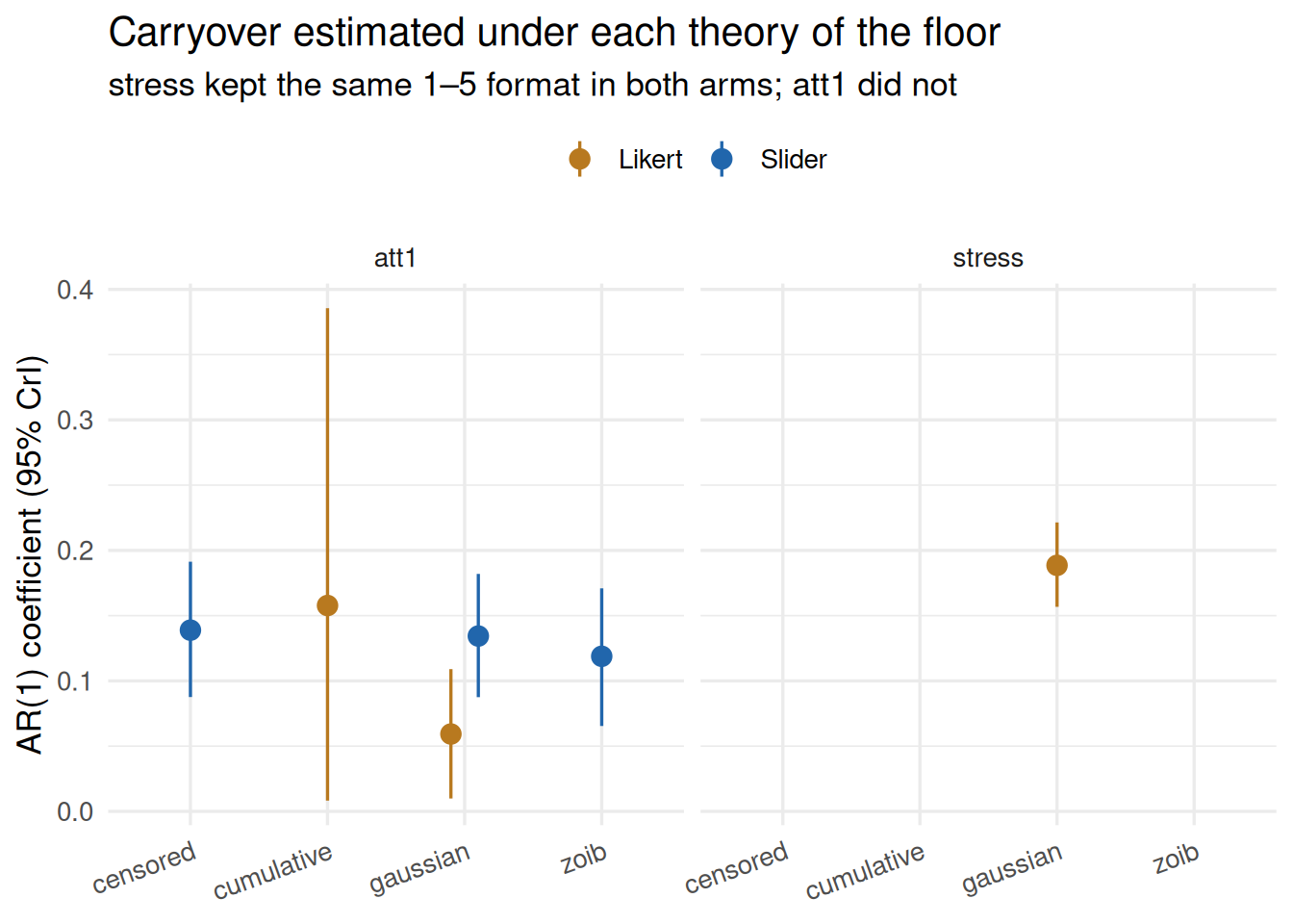
if (nrow(stage_b) >0&&"phi_ar1"%in%names(stage_b)) { d <- stage_b |>filter(!is.na(phi_ar1), converged)if (nrow(d) >0) {ggplot(d, aes(x = family, y = phi_ar1, colour = arm)) +geom_pointrange(aes(ymin = phi_ar1_lo, ymax = phi_ar1_hi),position =position_dodge(width = .4)) +facet_wrap(~ item) +scale_colour_manual(values =c("Likert"= irw_amber, "Slider"= irw_blue),name =NULL) +labs(x =NULL, y ="AR(1) coefficient (95% CrI)",title ="Carryover estimated under each theory of the floor",subtitle ="stress kept the same 1–5 format in both arms; att1 did not") +theme(legend.position ="top",axis.text.x =element_text(angle =20, hjust =1)) }}
Figure 4
Warning4 fit(s) did not mix
The chains disagree (Rhat above 1.01): att1 / Likert / censored (Rhat 2.87, ESS 2); stress / Likert / censored (Rhat 2.24, ESS 3); stress / Slider / censored (Rhat 2.13, ESS 3); stress / Slider / cumulative (Rhat 1.01, ESS 199). These are excluded from the figure, so read a gap there as ‘would not estimate’ rather than ‘was not tried’. Failure to converge is not proof that a model is wrong — but a model that will not estimate on the data it is recommended for is a practical result in its own right.
Note1 fit(s) mixed but were under-sampled
stress / Likert / cumulative (Rhat 1.009, ESS 260). These are a different situation from the ones above: the chains agree, there are simply too few effective draws at draft settings. More iterations would fix them, and they are excluded from the figure only out of caution, not because the model failed.
Note1 fit(s) had divergent transitions
Divergences are reported separately from mixing because they mean something different: the sampler failed to explore part of the posterior even where Rhat and effective sample size look healthy, so the estimate may be biased rather than merely imprecise. These fits are kept in the figure — discarding them would bias the comparison toward the families that happen to sample easily — but the Div. column is the honest caveat on any number in their rows.
Across the fits that converged, the carryover coefficient moves by up to 0.098 between model families on the same data (att1, Likert arm). The carryover parameter is not invariant to a modelling choice the field usually makes by convention.
More consequentially, the correlation between a person’s mean level and their innovation variance changes sign depending on which theory of the floor is adopted — in att1 (Likert arm), -0.145 to 0.260; att1 (Slider arm), -0.290 to 0.090. That is the parameter the preprint reports as biased when the floor is ignored. These estimates come from converged fits on identical data, differing only in what the model assumes a floor to be. A reader who picks one family and reports the correlation would conclude that people with higher average levels are more variable, or less, depending on that choice alone.
Can the censored model even be fitted?
The sharpest result here is not an estimate but an outcome. att1 was administered as a five-point item to one randomised arm and as a slider to the other, with the same protocol and schedule. The censored model — the remedy the preprint recommends — was fitted to both.
Code
if (nrow(stage_b) >0&&"rhat_ar"%in%names(stage_b)) { ce <- stage_b |>filter(family =="censored") |>transmute(Item = item, Arm = arm, `Categories`= n_cat,`At floor (%)`=round(floor_pct, 1),Rhat =round(rhat_ar, 3), ESS =round(ess_ar),`Minutes`=round(mins, 1),Estimable =ifelse(converged, "yes", "**no**"))if (nrow(ce) >0) kable(ce, caption ="The censored model, by response format.")}
Table 5: The censored model, by response format.
Item
Arm
Categories
At floor (%)
Rhat
ESS
Minutes
Estimable
att1
Likert
5
21.5
2.866
2
96.4
no
att1
Slider
101
7.9
1.001
1698
4.2
yes
stress
Likert
5
29.6
2.235
3
110.1
no
stress
Slider
5
40.0
2.128
3
34.7
no
Of the censored fits attempted so far, 1 of 1 on a near-continuous response converged, and 0 of 3 on a five-point response did.
The ordinal failures are not marginal: att1/Likert reached Rhat 2.87 with bulk ESS 2 after 96 minutes; stress/Likert reached Rhat 2.24 with bulk ESS 3 after 110 minutes; stress/Slider reached Rhat 2.13 with bulk ESS 3 after 35 minutes.
One row separates response format from the people in each arm. stress kept its five-point format in the slider arm — it was never converted — so those participants were randomised into the slider condition while still answering an ordinal item. The censored model fails there too (Rhat 2.13, bulk ESS 3), exactly as it does in the Likert arm. Had it failed only among Likert-arm participants, those participants would have been a rival explanation. They are not: it is the item’s response format that decides, not the arm.
That count needs one qualification before it can be read as being about censoring. A censored failure only implicates censoring if some other family managed the same rows. In 2 of 2 ordinal cells where another family did converge, the censored model did not — so there the failure is specific to it. But in 1 ordinal cell (stress/Slider, 40% at floor) no model converged at all — not the censored one, not the graded one, not even the naive Gaussian, which exhausted its time budget. That cell is evidence that a severe floor is hard for everything, and it is not evidence about censoring in particular. Counting it toward the censored tally would overstate the case.
This is what the censoring assumption predicts about itself. A censored model says the observed floor conceals a continuum extending below it. On a slider that is a coherent claim. On a five-point item there is nothing below category one, and the likelihood must place mass in a region the response format does not have — so the sampler cannot settle. Randomisation is what makes this readable: participants did not choose their response format.
Note that floor mass does not explain the split. The ordinal items carry 21.5% and 40.0% of responses at the floor and both fail; the continuous item carries 7.9% and converges in 4 minutes. It is the number of categories beneath the floor, not the amount of mass sitting on it, that decides whether the model can be estimated at all.
What is robust, and what is not
Within a cell, the carryover coefficient moves across families by 0.000 to 0.098, while the mean-dispersion correlation moves by 0.000 to 0.405. The correlation changes sign in 2 of 3 cells. The asymmetry is the point: carryover survives a change in what you assume the floor to be, and the parameter the preprint is concerned with does not.
Where all three are estimable, censoring is the outlier
Code
if (nrow(stage_b) >0) { full <- stage_b |>filter(converged) |>group_by(item, arm) |>filter(n() >=3) |>ungroup()if (nrow(full) >0) { full |>transmute(Item = item, Arm = arm, Model = family,`At floor (%)`=round(floor_pct, 1),Carryover =round(phi_ar1, 3),`cor(mean, disp)`=round(cor_mean_disp, 3)) |>arrange(Item, Arm, Model) |>kable(caption ="Cells where every admissible family converged.") }}
Table 6: Cells where every admissible family converged.
Item
Arm
Model
At floor (%)
Carryover
cor(mean, disp)
att1
Slider
censored
7.9
0.139
-0.290
att1
Slider
gaussian
7.9
0.134
0.090
att1
Slider
zoib
7.9
0.119
0.027
In every cell where all three admissible families converge, the model furthest from the others on the mean-dispersion correlation is censored. That matters for how the preprint’s recommendation reads. Comparing only a naive Gaussian against a censored model, the censored estimate looks like a correction — it is the one that moved. With a third, independently motivated treatment of the boundary in the comparison, the naive and inflated-beta estimates sit close together and the censored one sits apart. Being the estimate that moves is not the same as being the estimate that is right, and two models are not enough to tell those apart.
This section exists because reviewers of the scoping brief argued that an appropriate link should be compared against censoring rather than assumed away. With only the two models the page originally proposed, the distinction above could not have been seen.
Limitations
There is no predictive-fit comparison here, and that is deliberate. Two independent problems rule it out. First, the families are not fitted to the same response representation: Gaussian and censored models use a standardised continuous response, the cumulative model an ordinal probability mass function, the inflated beta a density on the unit interval. Log-densities across those are not on a common scale, so a “best fit” ranking would be meaningless whatever the numbers said.
Second, and decisively, PSIS-LOO breaks down on these models. The censored fit reported 1,516 of 1,692 observations with a Pareto k above 0.7 — the importance-sampling approximation has failed for almost every observation, which is what one should expect when each observation carries its own person-level location and scale parameters. An elpd column was computed and then removed from this page rather than shown with a caveat, because a number that cannot be trusted is not improved by a footnote. The comparison below therefore rests on the parameter estimates, not on out-of-sample fit.
The dispersion parameter is not the same object across families. The Gaussian and censored models have a residual standard deviation; the inflated beta has a precision, and the cumulative model a discrimination. Their person-level correlations with the intercept play analogous roles but are not numerically the same quantity, so the cor(mean, dispersion) column should be read for sign and rough magnitude, not compared digit for digit. The AR(1) coefficient is comparable across all four, which is why it carries the headline. This is a real obstacle to the preprint’s framing, not just to ours: the parameter it reports as biased is defined inside a Gaussian latent-variable metric, and the alternatives a reader might reach for do not all have one.
The format contrast is between persons. Randomisation makes it a fair comparison, but it is not the within-person crossing that would let us hold the participant fixed. The stress item mitigates this — same format in both arms, so arm differences on it are attributable to sample rather than format — but one control item is not a full design.
These are bipolar scales. Both the Likert (−2…5) and slider (−50…100) items run from a negative to a positive pole, so the “floor” is an extreme negative response, not the absence of a symptom. The preprint’s motivating case — depression and anxiety ESM, where the floor means “no symptoms today” and is very common — is the unipolar situation. The ordinal tables in the pool above include that case; vollbracht does not. Results here should not be read as settling what happens on a unipolar symptom scale.
Response direction is not harmonised in IRW. “Floor” throughout means the observed minimum of that item. For a reverse-keyed item that is the substantive ceiling. This is reported as found rather than silently corrected, because recovering the intended keying reliably is its own problem.
Carryover is a lagged predictor, not a residual AR process. The first version of this page used brms’s ar() term. It builds a per-group residual autocorrelation matrix, and combined with the person-varying sigma that the preprint’s target parameter requires, it was both badly identified and extremely slow — Rhat 1.41, bulk effective sample size 5, and 147 minutes for a single fit. The lagged-predictor form above is what DSEM actually specifies, is far cheaper, and yields a carryover coefficient comparable across response families in a way an ar[1] parameter is not. One consequence to keep in mind: \(\phi\) here is a population-level coefficient. DSEM typically lets it vary by person, and that random slope is not fitted here.
Divergent transitions are reported, not screened away. Some fits sample cleanly and some produce divergences even at adapt_delta = 0.99. A divergence is not the same failure as poor mixing: it says the sampler could not explore part of the posterior, so an estimate can be biased while still looking precise. Dropping the affected fits would have quietly biased the comparison toward the families that happen to sample easily — precisely the families the page is trying to compare — so they are kept and the count is printed alongside every estimate.
The target parameter is hard to estimate at ESM sample sizes. The first draft run of this page produced Rhat 1.8, a bulk effective sample size of 3, and 416 divergent transitions on a fit that nonetheless reported a tight-looking interval. The location-scale structure the preprint’s parameter requires — each person’s mean correlated with their own residual variability — is only weakly identified with tens of people and tens of occasions, and flat priors leave the sampler nowhere to stand. The fits here use weakly informative priors, a standardised response, and adapt_delta = 0.99. Convergence is reported per fit rather than assumed, and non-converging fits are excluded from the figure. This is a practical caveat on the preprint’s recommendation as much as on this page: a model can be the right one and still be beyond what the data will support.
Reproducibility
Computed on 2026-09-09, profiling 26 of 26 candidate tables.
Run Rscript vignettes/esm_floor_compute.R from the repository root, with REDIVIS_API_TOKEN set to a read-scoped token. The script caches every table profile and every model fit separately under esm_floor_data/fits/, so an interrupted run resumes rather than restarting.
We thank Lijin Zhang and Esther Ulitzsch, who helped design this page and reviewed it. The draft asked whether censoring or an ordinal artefact explains a floor; their reading is why it now treats censoring as one of three theories of what a floor is, alongside an appropriate link that models the boundedness directly and a graded model under which the floor was never special. Errors that remain are ours.
Molenaar, Dylan, Mariana C’uri, and Jorge L. Baz’an. 2022. “Zero and One Inflated Item Response Theory Models for Bounded Continuous Data.”Journal of Educational and Behavioral Statistics 47 (6): 693–735. https://doi.org/10.3102/10769986221108455.
Vollbracht, D., C. Ottenstein, and S. Ecker. 2026. “Slider Versus Likert Scales: Psychometric Properties in Ambulatory Assessment.”Behavior Research Methods 58: 97. https://doi.org/10.3758/s13428-026-02992-4.