Bounded Continuous Responses: Comparing Beta IRT, Samejima’s CRM, and Mueller’s CRSM

Slider and visual-analogue-scale items produce a response that is continuous but lives in a fixed, interpretable range, like [0,1] or [0,100] – not the open-ended continuous case standard CFA/linear-factor models assume. We compare four published ways of modeling that: a naive linear baseline that ignores the bounds, Noel and Dauvier’s Beta IRT model, Samejima’s Continuous Response Model, and Mueller’s Continuous Rating Scale Model, on one simulated dataset and one real IRW table.

Published

August 2, 2026

Note

This vignette — including the dataset search, the compute script, the analysis design, and the writing below — was produced largely by Claude (Anthropic), working from a task specification and with human review. Treat the methodological choices and interpretations accordingly, and check the compute script (continuous_bounded_compute.R) directly if you’re relying on the numbers here.

Motivation

Visual analogue scales, slider ratings, and continuous confidence or percentage judgments are common: a respondent marks a point on a fixed, labeled segment (0 to 100, say), and the raw response is a continuous number that is bounded at both ends. This is a different measurement problem from the unbounded continuous case (response times, open-ended magnitude estimates), which reduces to standard linear-factor or CFA modeling and is covered elsewhere on this site – the bounds themselves are the interesting part here, because they create floor/ceiling effects and non-constant response variance near the edges that a plain linear model doesn’t see.

Three published models handle this directly. Noel and Dauvier’s Beta IRT model (Noël and Dauvier 2007) treats the response as Beta-distributed given ability, with the two natural Beta parameters reparameterized into an item difficulty and a dispersion. Samejima’s Continuous Response Model (Samejima 1973) models a monotonic transform of the response as normal given ability – the historically original approach, predating Beta IRT by over 30 years. Mueller’s Continuous Rating Scale Model (Müller 1987) takes a Rasch-family, specific-objectivity approach, estimated by pairwise conditional likelihood; Verhelst’s (2019) exponential family framework (Verhelst 2019) is the modern theoretical generalization of Mueller’s model, though the model actually fitted here is Mueller’s original. We compare these three against a naive linear (Gaussian, identity-link) baseline that ignores the bounds entirely – the “what if you just treat it like ordinary continuous data” control, playing the same role the Rasch baseline plays in the site’s guessing-models vignette.

Data and methods

The four core specs

  1. Naive linear baseline – single-factor CFA via lavaan, identity link, Gaussian residual, fit directly on the raw (rescaled-to-[0,1]) response. Ignores boundedness entirely.
  2. Beta IRT (Noël and Dauvier 2007) – fit as a discretized custom mirt itemtype wrapping sirt::brm.irf(), following sirt’s own documented mirt-estimation recipe (?sirt::brm.sim). Two variants: item-varying dispersion (each item gets its own dispersion parameter, the model’s default parameterization) and fixed dispersion (one dispersion parameter shared across all items, via an mirt parameter constraint).
  3. Samejima’s Continuous Response Model (Samejima 1973)EstCRM::EstCRMitem() / EstCRMperson().
  4. Mueller’s Continuous Rating Scale Model (Müller 1987) – a patched copy of pcIRT::CRSM() / a from-scratch reimplementation of its person-scoring equation (see Limitations for why patching was necessary).

Model equations

Each spec below is written exactly as it is fit in the compute script – same parameter names, same functional form – so the equations here can be checked directly against continuous_bounded_helpers.R. Ability \(\theta_i\) itself is never bounded – every widget below spans \(\theta\in[-3,3]\) – it is only the response \(X_{ij}\) that each model constrains (or, for the naive baseline, fails to constrain) to \([0,1]\). Each equation is followed by a small widget plotting that model’s own \(E[X_{ij}\mid\theta_i]\) curve, so you can see what the equation implies before any fitting happens; dispersion parameters that don’t have their own slider are held fixed at a representative value, noted in each case.

Naive linear baseline. Ordinary single-factor CFA on the raw (rescaled-to-\([0,1]\)) response: \(X_{ij} = \nu_j + \lambda_j\theta_i + \varepsilon_{ij}\), \(\varepsilon_{ij}\sim N(0,\sigma_j^2)\), fit via lavaan::cfa(). Nothing here constrains \(X_{ij}\) to \([0,1]\), as the widget below makes obvious once \(\theta\) moves far enough from \(b\).

Beta IRT (Noël and Dauvier 2007), as sirt::brm.irf() actually parameterizes it: \(X_{ij}\mid\theta_i \sim \text{Beta}(\text{shape1}_{ij}, \text{shape2}_{ij})\), with \[\text{shape1}_{ij} = \exp\!\left(\frac{\theta_i-\delta_j+\tau_j}{2}\right), \qquad \text{shape2}_{ij} = \exp\!\left(\frac{-\theta_i+\delta_j+\tau_j}{2}\right),\] where \(\delta_j\) is item difficulty and \(\tau_j\) is dispersion (fixed across items in the “fixed dispersion” variant, free in the “item-varying” variant). Working out this Beta distribution’s mean shows it reduces exactly to \(E[X_{ij}\mid\theta_i] = \text{logistic}(\theta_i-\delta_j)\), independent of \(\tau_j\)there is no discrimination parameter, so unlike the other 3 widgets on this page, this one has only a single slider. \(\tau_j\) is left out of it entirely, not just discrimination: since \(\tau_j\) enters \(\text{shape1}_{ij}\) and \(\text{shape2}_{ij}\) with the same sign, it changes their sum (the Beta distribution’s concentration) without changing their ratio (the mean), so it would have no visible effect on this mean-curve widget either. It does change the density’s spread, though – see the \(\tau_j\) slider in Comparing response densities across models below.

Samejima’s Continuous Response Model (Samejima 1973), via EstCRM::EstCRMitem(): the raw response is transformed to \(Z_{ij}=\ln\!\big(X_{ij}/(1-X_{ij})\big)\), and \(Z_{ij} = \alpha_j(\theta_i - b_j) + e_{ij}\), \(e_{ij}\sim N(0,\sigma_j^2)\), i.e. an ordinary linear factor model on the transformed scale. \(\alpha_j\) is discrimination and \(b_j\) is difficulty. The observed-scale mean response is the backtransform of this normal model’s mean through the logistic link (dispersion held fixed at \(\sigma=1\) below).

Mueller’s Continuous Rating Scale Model (Müller 1987), via pcIRT::CRSM(): a Rasch-family (specific-objectivity) density, \[f(x_{ij}\mid\theta_i) \;\propto\; \exp\!\big[x_{ij}(\theta_i-b_j) + x_{ij}(1-x_{ij})\lambda_j\big], \quad x_{ij}\in[0,1],\] with a single item-location parameter \(b_j\) and a dispersion parameter \(\lambda_j\) – no discrimination parameter, by construction of the Rasch-family specific-objectivity property. Unlike Beta IRT, \(\lambda_j\) does move the mean here (the widget below lets it, rather than holding it fixed), since the backtransform from the exponential-tilt density to \(E[X_{ij}\mid\theta_i]\) is nonlinear in \(\lambda_j\).

Comparing response densities across models

The 4 widgets above each plot a single line – a model’s mean response – but every one of them is really a full probability distribution over \(X_{ij}\in[0,1]\) (or, for naive linear, over all of \(\mathbb{R}\)). Because all 4 responses live on the same \([0,1]\) scale, their densities can be overlaid directly. Rather than fix \(\theta\) at a specific, unbounded value, the slider below is expressed as an ability percentile, mapped to \(\theta\) through the standard normal quantile function – the same \(\theta_i\sim N(0,1)\) assumed everywhere else in this vignette (e.g. the simulation grid’s theta_true <- rnorm(N)). 50% is \(\theta=0\), i.e. the person of average ability the earlier fixed value silently assumed; dragging toward the tails reaches every \(\theta\) a percentile-bounded slider can, without the awkwardness of a slider whose bounds are themselves an arbitrary choice on an unbounded scale. Dispersion is held at the same representative values used above (\(\sigma=0.15\) for naive linear on the raw scale, \(\sigma=1\) for Samejima CRM, \(\lambda=2\) for Mueller CRSM); drag difficulty (\(b\)) and discrimination (\(a\), Beta IRT’s \(\delta_j\) and Mueller CRSM have no discrimination term) to see how each model’s whole distribution, not just its mean, responds. Beta IRT gets one more slider here than in its own widget above: \(\tau_j\), which has no effect on Beta IRT’s mean curve (see Model equations) but a real one on its density’s concentration, visible only in a density view like this one.

The dashed vertical lines at \(x=0\) and \(x=1\) mark the response range; naive linear (dashed gray) is the only density that isn’t actually confined inside them – exactly the failure mode its widget above shows for the mean curve, now visible in the distribution itself. The other 3 densities all integrate to 1 strictly within \([0,1]\): Beta IRT’s shifts left/right with \(\delta_j\) without changing shape, but narrows or widens in place as \(\tau_j\) moves – large \(\tau_j\) concentrates it tightly around the mean, small (or negative) \(\tau_j\) spreads it out and can even pull mass toward both boundaries at once, all while the mean itself never moves, exactly as the equation in Model equations implies. Samejima CRM’s and Mueller CRSM’s shapes visibly skew as \(b\) moves them toward either boundary, a consequence of the nonlinear backtransform in both models that a mean-curve-only view can’t show. Moving \(a\) redistributes naive linear’s and Samejima CRM’s mass without translating it (steeper slope on the same \(\theta\)), and does nothing to Beta IRT’s or Mueller CRSM’s density, consistent with neither model having a discrimination parameter.

Estimation and model comparison

Every model’s held-out fit is reported as the log-probability of the response falling in a small interval, not a raw point density. This choice exists because the 4 models don’t report likelihood on the same scale to begin with: reading EstCRM::EstCRMitem()’s source shows it transforms the raw response to \(Z = \ln\!\big(X/(K-X)\big)\) and computes its entire EM log-likelihood on that transformed scale, not the original response scale the Beta IRT and naive linear fits use. Comparing those two log-likelihoods directly would be comparing different units – like comparing an error reported in inches to one reported in centimeters without converting first. The usual fix is a model-specific Jacobian correction; instead, every model’s held-out score here is \(\log P(\text{bin}_{lo} < X < \text{bin}_{hi})\), using the same bin edges (on the raw, rescaled-to-\([0,1]\) scale) for all 4 models. A probability that a response lands in a fixed interval means the same thing regardless of which internal scale a model uses to compute it, so this sidesteps the rescaling problem entirely rather than requiring a per-model correction.

Held-out log-probability, built this way, is the metric used to compare all 4 specs throughout this vignette. It’s a standard, interpretable scale for predictive fit, though not a validated best-practice specific to this bounded-continuous setting – flagged as an ad hoc choice worth revisiting (see Limitations).

This same design also makes scores comparable across the 11 real tables, not just across the 4 models within a table – a separate problem the rescaling was never explicitly built for but solves anyway. rescale01() maps every table’s raw response to \([0,1]\) using that table’s own bounds before anything else happens (continuous_bounded_helpers.R), and the bin edges used for scoring are equal-width on that shared \([0,1]\) scale with the same bin count (\(K=6\)) for every table, regardless of its raw range. A table scored on a raw 0-10 scale and one scored on a raw 0-100 scale both get bin width exactly \(1/6\) in the space the score is actually computed in – so a wide bar or point for one table isn’t wider raw units in disguise, and height differences across tables in the figures below reflect genuine differences in predictive fit, not unit mismatches.

Held-out design: genuine missing-response prediction

The project’s usual convention for held-out evaluation on IRW data is a response-level (missing-cell) holdout: mask a random subset of person x item cells, fit on the rest, score the masked cells. Fitting item parameters this way isn’t viable for 2 of the 4 specs – reading EstCRM::EstCRMitem() and pcIRT::CRSM()’s fitting code directly shows neither has any missing-data handling at all (both do matrix/pairwise algebra that silently breaks with NA cells, confirmed by testing) – so item parameters for all 4 specs are still fit on a complete training-person matrix, no missing cells.

Scoring, once item parameters are fixed, is a different matter: all 4 specs’ person-location estimators turn out to be NA-tolerant. mirt::fscores(response.pattern = ...) handles missing cells natively (a core mirt feature, not something added here); lavaan::lavPredict() computes factor scores from an incomplete newdata row the same way; EstCRM::EstCRMperson() skips NA columns per person when forming its theta estimate (confirmed by reading its source); and the from-scratch Mueller CRSM person-scoring routine (see Limitations) was written to do the same. Each was smoke-tested directly (masked vs. full-data theta estimates, correlation \(>0.98\) in every case) before being used for real.

That makes true cell-level prediction possible after all: for every held-out test person, a random subset of their items (25%, clamped to at least 1 kept and at least 1 held out) is hidden before estimating that person’s ability from the remaining items alone, and only the hidden items are scored. The model never sees the scored value, directly or indirectly, at any stage – this is genuine missing-response prediction, not the weaker “estimate ability from a person’s full vector, then score those same items” self-consistency check an earlier version of this design used.

Simulation

Before turning to real IRW tables, this section checks the 4 specs against data simulated directly from known, correctly-specified generating models – design first, then results. The short version, expanded below: every correctly-specified model recovers its true item parameters cleanly, the 3 bounded-response models beat the naive linear baseline on held-out log-probability regardless of which of them generated the data, and boundary inflation degrades every spec somewhat but the 3 bounded-response models noticeably less than naive linear. Real-data selection and results follow in the next section, once this baseline is established.

Design

A single illustrative condition (\(N=300\), \(J=10\), Beta IRT DGP, fixed dispersion) is shown first below, generated directly from the Beta IRT model’s own equations (sim_beta_irt() in continuous_bounded_helpers.R – a bug-fixed reimplementation of sirt::brm.sim()’s logic; see Limitations for why the reimplementation was necessary).

The full recovery/misspecification grid cross-fits all 4 core specs against 3 DGPs, generated from each model’s own equations: Beta IRT (sim_beta_irt()), Samejima CRM (sim_samejima_crm(): \(Z_{ij} = \alpha_j(\theta_i - b_j) + e_{ij}\), \(e_{ij}\sim N(0,\sigma_j^2)\), then \(X_{ij}=1/(1+e^{-Z_{ij}})\) – the exact inverse of EstCRM’s own \(Z=\ln(X/(1-X))\) transform), and Mueller CRSM (sim_muller_corsm(): grid-based inverse-CDF sampling from the same \(\exp[x(\theta-b)+x(1-x)\lambda]\) density used for scoring, since no closed-form sampler exists for this family). The naive-linear DGP is skipped: an unbounded-Gaussian DGP clipped to \([0,1]\) to make it “bounded” would introduce an artificial boundary spike unrepresentative of what a linear model actually generates.

Grid: \(N\in\{300,1000\}\), \(J\in\{8,20\}\), and, for the Beta IRT DGP specifically, fixed vs. item-varying dispersion – 8 + 4 + 4 = 16 conditions, plus 1 boundary-inflation condition (10% of responses forced to exactly 0, 10% forced to exactly 1, layered on the Beta IRT DGP at \(N=300\)/\(J=8\)) for 17 total. Run via furrr::future_pmap() + plan(multisession), cached separately from the real-data results below (own skip-if-exists gate in the compute script).

Does the correctly-specified model win, and does it recover parameters?

Code
if (cache_ok) {
  res$sim$scores |>
    mutate(model = factor(model, levels = names(model_colors))) |>
    ggplot(aes(x = model, y = mean_ll, fill = model)) +
    geom_col(width = 0.6) +
    geom_text(aes(label = sprintf("%.2f", mean_ll)), vjust = 1.4, color = "white", size = 3.5) +
    scale_fill_manual(values = model_colors, labels = model_labels, guide = "none") +
    scale_x_discrete(labels = model_labels) +
    labs(x = NULL, y = "Mean held-out log-probability (per response)",
         title = "Simulated Beta-IRT data: held-out fit by model") +
    theme(axis.text.x = element_text(angle = 20, hjust = 1))
} else {
  cat("Cache not found -- run continuous_bounded_compute.R first.")
}
Figure 1

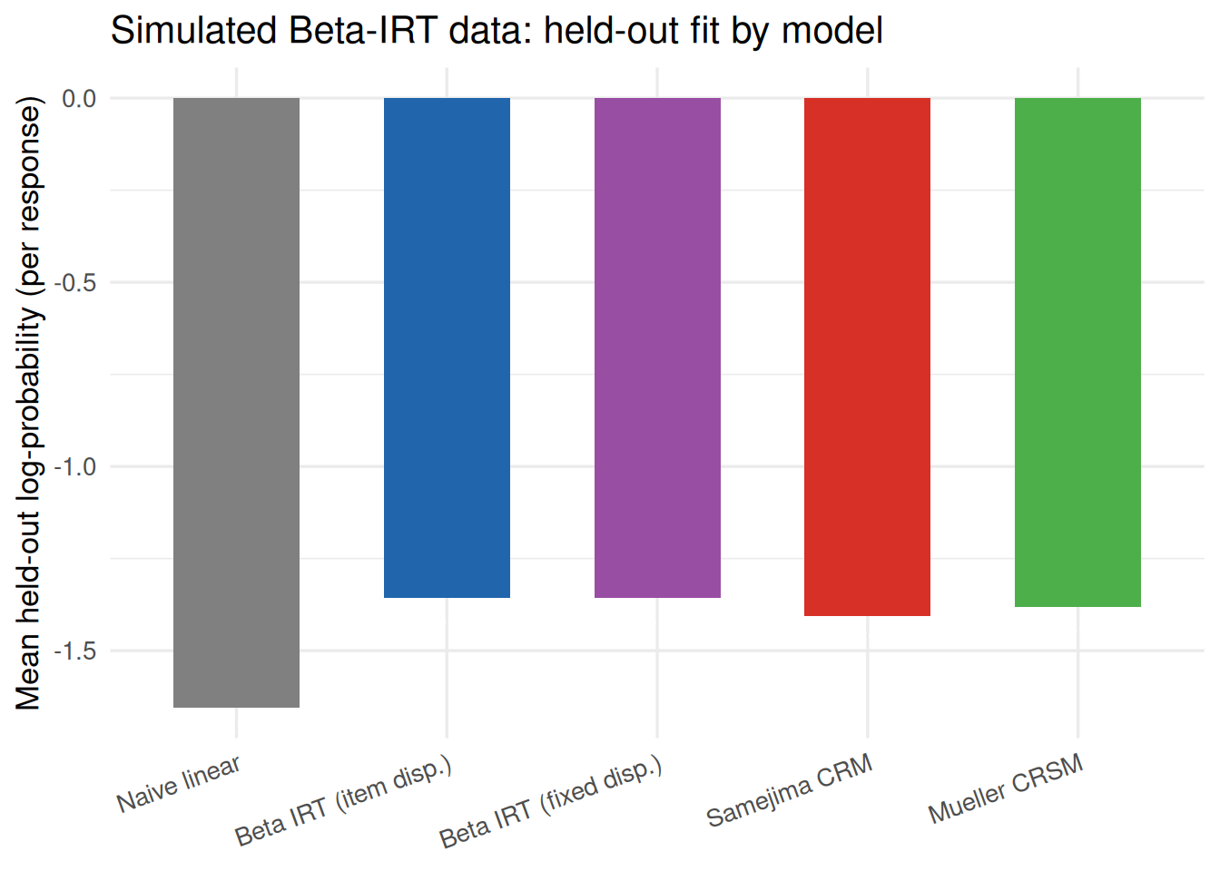
On data simulated directly from the Beta IRT model, the two Beta IRT variants have the best (least negative) held-out fit, essentially tied with Samejima CRM and Mueller CRSM, and all three clearly beat the naive linear baseline. This is the expected pattern for a correctly-specified-model recovery check: the models built for bounded continuous responses recover the truth better than the one that ignores the bounds.

Item-difficulty recovery for the item-varying-dispersion Beta IRT fit (correlation between estimated and true \(\delta\)) was 0.997.

The full recovery grid: 16 conditions x 3 DGPs

“Recovery” here means one specific, narrow comparison: for each condition, only the fitted model that matches that condition’s DGP is checked – the correlation between its estimated item-difficulty parameters and the true difficulties used to simulate the data (e.g. for a Beta-IRT-generated condition, only the Beta IRT fit’s estimated \(\delta_j\) vs. true \(b_j\) is computed). The other 3 fitted models aren’t included in this table at all: their difficulty-type parameters aren’t on a directly comparable scale to the true simulation parameters without a model-specific transform, so a recovery correlation for them isn’t computed here. (Whether all 4 models can nonetheless fit the same data well is a separate question, answered by the cross-fitting comparison just below, not by this table.) With that scope in mind, parameter recovery for the correctly-specified model was excellent everywhere – every one of the 16 non-inflation conditions recovered its true item parameters at \(r>0.96\), most above \(r>0.99\):

Code
if (grid_cache_ok) {
  grid_res$scores |>
    filter(!boundary_inflation, !response_heaping) |>
    distinct(dgp, N, J, dispersion_mode, recovery_cor) |>
    arrange(dgp, N, J, dispersion_mode) |>
    mutate(recovery_cor = sprintf("%.3f", recovery_cor)) |>
    knitr::kable(col.names = c("DGP", "N", "J", "Beta IRT dispersion", "Recovery r (correctly-specified model only)"))
} else {
  cat("Grid cache not found -- run continuous_bounded_compute.R first.")
}
Table 1
DGP N J Beta IRT dispersion Recovery r (correctly-specified model only)
beta_irt 300 8 fixed 0.998
beta_irt 300 8 item 0.992
beta_irt 300 20 fixed 0.995
beta_irt 300 20 item 0.995
beta_irt 1000 8 fixed 0.999
beta_irt 1000 8 item 0.999
beta_irt 1000 20 fixed 0.998
beta_irt 1000 20 item 0.999
muller_corsm 300 8 NA 0.973
muller_corsm 300 20 NA 0.961
muller_corsm 1000 8 NA 0.991
muller_corsm 1000 20 NA 0.986
samejima_crm 300 8 NA 0.999
samejima_crm 300 20 NA 0.990
samejima_crm 1000 8 NA 1.000
samejima_crm 1000 20 NA 0.999

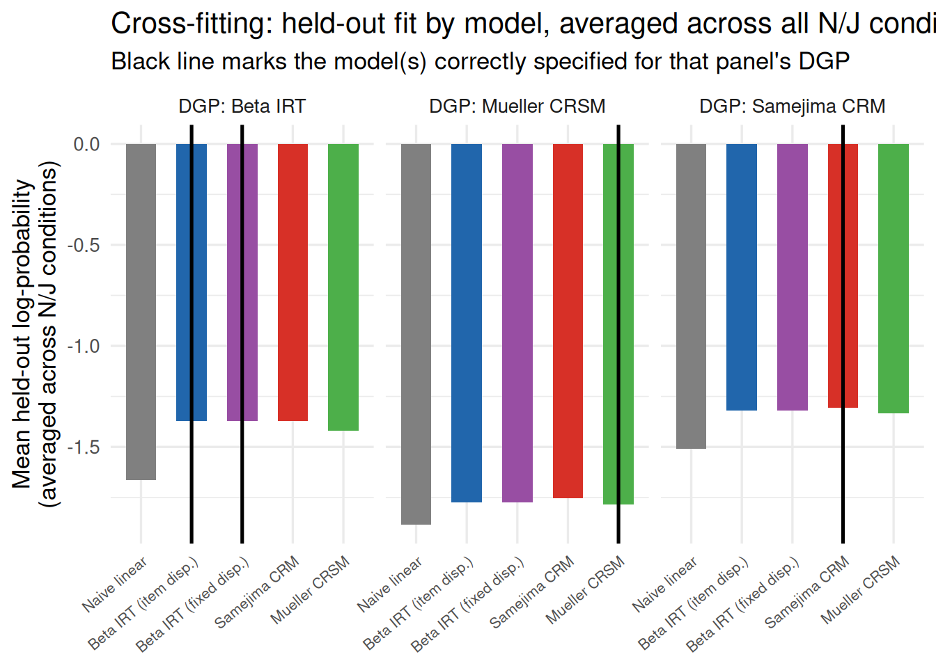
More useful than “does recovery work” (it does, everywhere) is the cross-fitting question: when data comes from one DGP, which of the 4 fitted specs wins the held-out comparison?

Code
if (grid_cache_ok) {
  # marks the correctly-specified model(s) in each DGP facet with a vertical
  # line; the Beta IRT DGP panel averages over both dispersion_mode
  # conditions, so both Beta IRT variants are correctly specified somewhere
  # in that average and both get a line
  correct_model_df <- data.frame(
    dgp_label = c("DGP: Beta IRT", "DGP: Beta IRT", "DGP: Samejima CRM", "DGP: Mueller CRSM"),
    model = factor(c("beta_irt_item_dispersion", "beta_irt_fixed_dispersion", "samejima_crm", "muller_corsm"),
                   levels = names(model_colors))
  )

  grid_res$scores |>
    filter(!boundary_inflation, !response_heaping) |>
    mutate(model = factor(model, levels = names(model_colors)),
           dgp_label = recode(dgp, beta_irt = "DGP: Beta IRT", samejima_crm = "DGP: Samejima CRM",
                               muller_corsm = "DGP: Mueller CRSM")) |>
    group_by(dgp_label, model) |>
    summarise(mean_ll = mean(mean_ll, na.rm = TRUE), .groups = "drop") |>
    ggplot(aes(x = model, y = mean_ll, fill = model)) +
    geom_col(width = 0.6) +
    geom_vline(data = correct_model_df, aes(xintercept = as.numeric(model)),
               color = "black", linewidth = 0.9) +
    scale_fill_manual(values = model_colors, labels = model_labels, guide = "none") +
    scale_x_discrete(labels = model_labels) +
    facet_wrap(~dgp_label, ncol = 3) +
    labs(x = NULL, y = "Mean held-out log-probability\n(averaged across N/J conditions)",
         title = "Cross-fitting: held-out fit by model, averaged across all N/J conditions per DGP",
         subtitle = "Black line marks the model(s) correctly specified for that panel's DGP") +
    theme(axis.text.x = element_text(angle = 40, hjust = 1, size = 8))
} else {
  cat("Grid cache not found -- run continuous_bounded_compute.R first.")
}
Figure 2

The pattern is consistent across all 3 DGPs, and, as shown in Real data below, the same pattern holds up on real IRW tables too: the 3 bounded-response models cluster tightly together and substantially outperform the naive linear baseline, regardless of which of the 3 actually generated the data. “Correctly specified wins” is a much weaker pattern here than under a self-consistency check, though: under the Beta IRT DGP, both Beta IRT variants edge out Samejima CRM by only $\(0.003 in mean held-out log-probability -- a three-way tie in practice. Under the Samejima CRM DGP, Samejima does come out slightly ahead, but by less than 0.01. And under the Mueller CRSM DGP, Mueller CRSM is **not** the best-fitting model -- Samejima CRM scores marginally better than Mueller's own generating model, a genuine (if small) misspecification surprise, not papered over here. The margin between the 3 bounded-response models is small compared to the gap to naive linear in every case -- these 3 models are more interchangeable with each other than any of them is with a model that ignores the bounds, but which one "wins" under true missing-response prediction is close to a coin flip. One fit failed outright: Samejima CRM's EM did not converge (a `missing value where TRUE/FALSE needed` error partway through) on one Mueller-CRSM-generated dataset (\)N=300$, \(J=8\)) – a real misspecification-robustness finding, not papered over; see Limitations.

Boundary inflation: does floor/ceiling piling break anything?

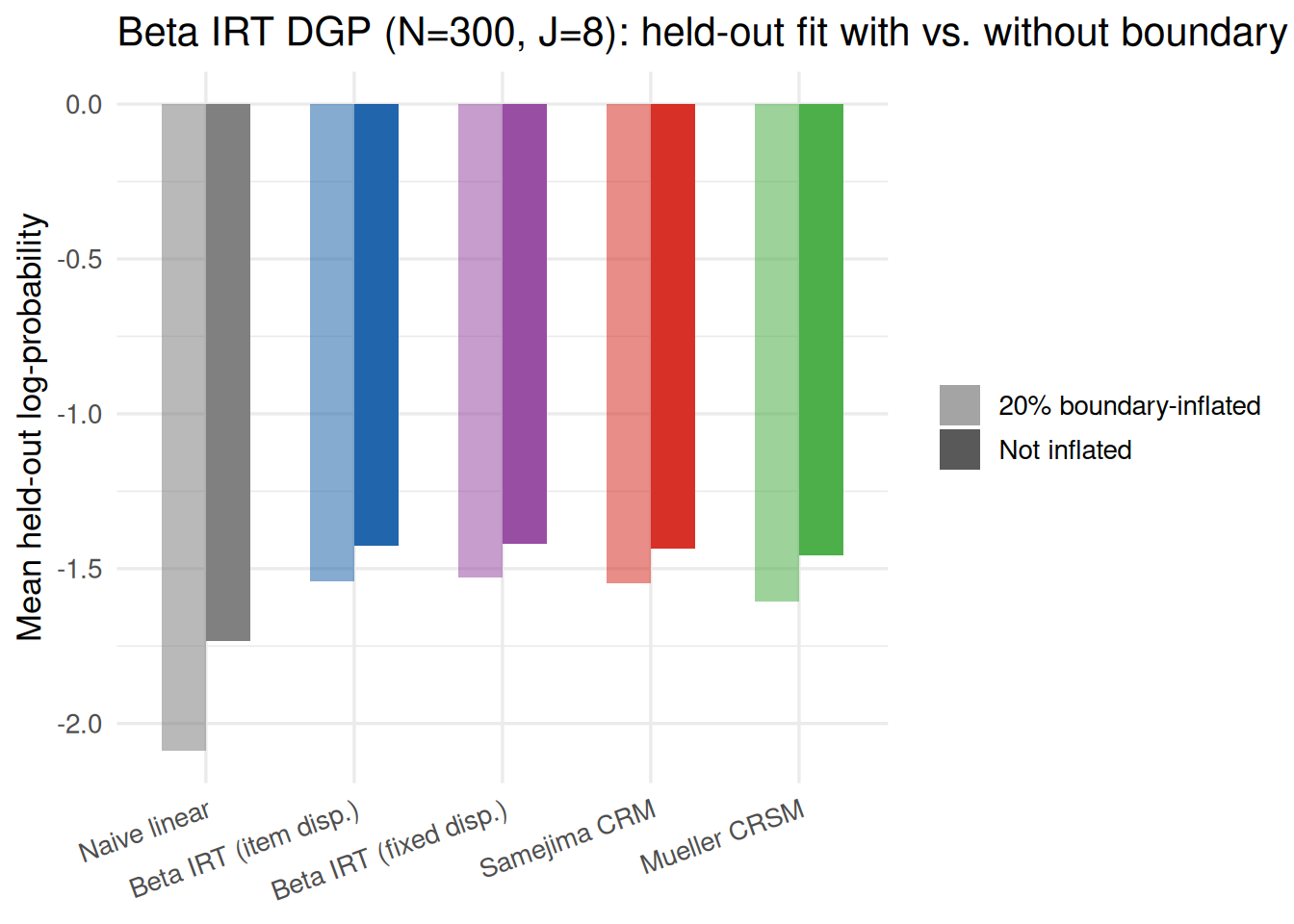
Beyond fitting, we asked how each of the 4 specs’ held-out fit degrades when 20% of responses are forced to the exact boundary (10% to 0, 10% to 1) on top of the Beta IRT DGP. This is a stress test of the 4 existing specs, not a new model: none of them includes a dedicated zero-one-inflated component, so the question is how much their held-out fit suffers without one, not which model handles inflation best.

Code
if (grid_cache_ok) {
  grid_res$scores |>
    filter(dgp == "beta_irt", N == 300, J == 8, dispersion_mode == "fixed", !response_heaping) |>
    mutate(model = factor(model, levels = names(model_colors)),
           condition = ifelse(boundary_inflation, "20% boundary-inflated", "Not inflated")) |>
    ggplot(aes(x = model, y = mean_ll, fill = model, alpha = condition)) +
    geom_col(position = "dodge", width = 0.6) +
    scale_fill_manual(values = model_colors, labels = model_labels, guide = "none") +
    scale_alpha_manual(values = c("Not inflated" = 1, "20% boundary-inflated" = 0.55), name = NULL) +
    scale_x_discrete(labels = model_labels) +
    labs(x = NULL, y = "Mean held-out log-probability",
         title = "Beta IRT DGP (N=300, J=8): held-out fit with vs. without boundary inflation") +
    theme(axis.text.x = element_text(angle = 20, hjust = 1))
} else {
  cat("Grid cache not found -- run continuous_bounded_compute.R first.")
}
Figure 3

Every spec’s held-out fit gets worse under inflation – none of the 4 core specs explicitly models a zero-one-inflated mixture, so this is expected – but not by the same amount. The naive linear baseline degrades by about 20% (mean log-probability drops from -1.74 to -2.09); the 3 bounded-response models degrade by roughly 8-10% each (e.g. Mueller CRSM: -1.46 to -1.61). The bounded-response models’ smooth density still puts more mass near the boundary than a Gaussian does, so they absorb some of the extra piling without a dedicated inflation term, while the naive linear model has nothing in its structure to absorb it at all. None of the 4 handle it well – a true zero-one-inflated extension (Molenaar et al. 2022) would be needed for that – but the bounded-response models are comparatively more robust to it than the baseline that ignores boundedness altogether.

Response heaping: does round-number clumping break anything?

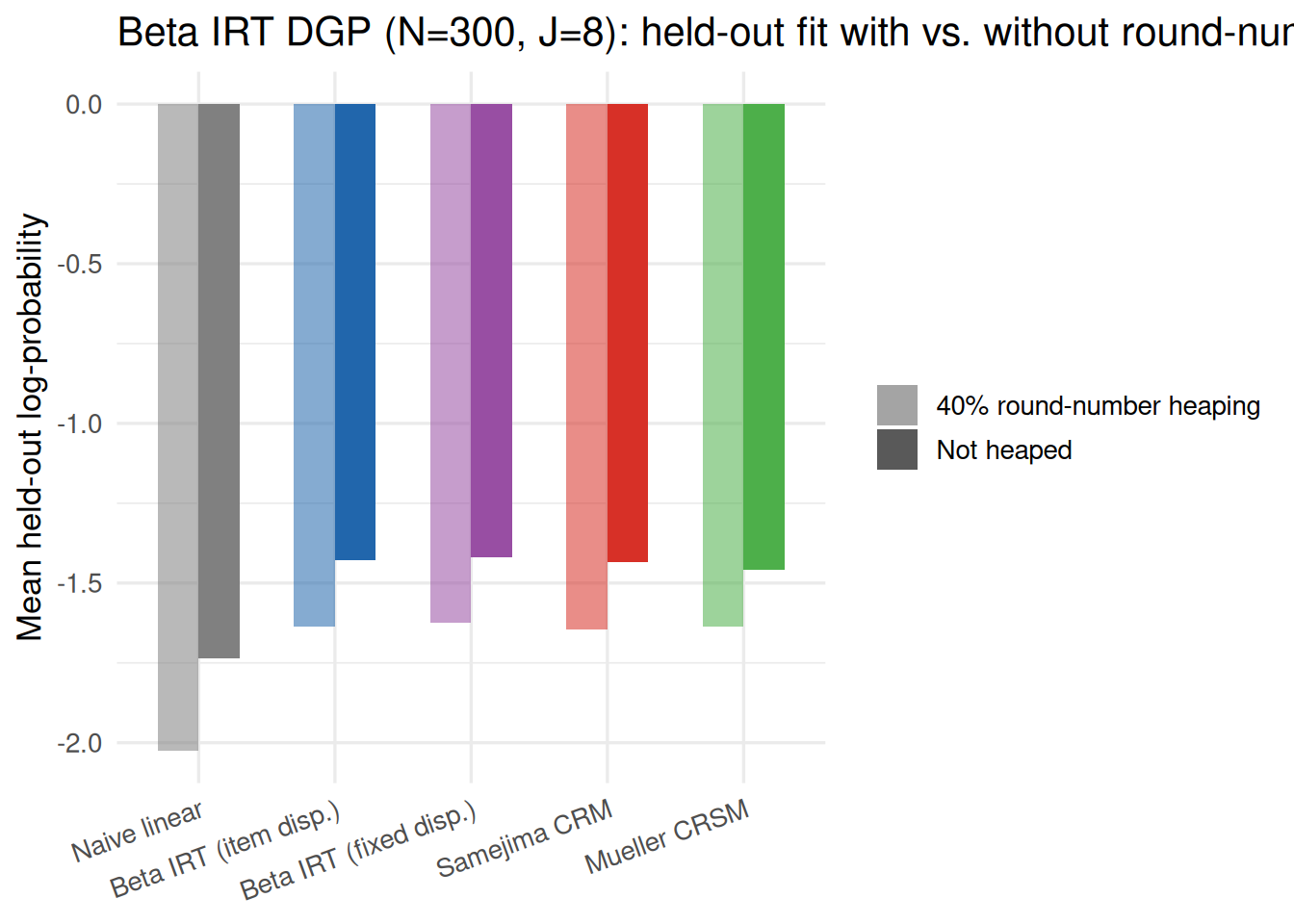
Boundary inflation isn’t the only way real responses depart from a smooth continuous distribution. As Real data below shows in detail, the primary real table’s responses heap not just at the scale ceiling but at the scale midpoint and quarter-points too – a multi-modal pattern no unimodal density, bounded or not, is built to represent. This condition tests that directly: with probability 0.4 per cell, sim_beta_irt()’s continuous draw is thrown away and replaced with a value drawn uniformly at random from 5 fixed points spanning the range (\(0, 0.25, 0.5, 0.75, 1\)), independent of the underlying \(\theta\) (apply_response_heaping() in continuous_bounded_helpers.R) – same base condition as boundary inflation above (\(N=300\), \(J=8\), Beta IRT DGP, fixed dispersion), so the two are directly comparable.

Code
if (grid_cache_ok) {
  grid_res$scores |>
    filter(dgp == "beta_irt", N == 300, J == 8, dispersion_mode == "fixed", !boundary_inflation) |>
    mutate(model = factor(model, levels = names(model_colors)),
           condition = ifelse(response_heaping, "40% round-number heaping", "Not heaped")) |>
    ggplot(aes(x = model, y = mean_ll, fill = model, alpha = condition)) +
    geom_col(position = "dodge", width = 0.6) +
    scale_fill_manual(values = model_colors, labels = model_labels, guide = "none") +
    scale_alpha_manual(values = c("Not heaped" = 1, "40% round-number heaping" = 0.55), name = NULL) +
    scale_x_discrete(labels = model_labels) +
    labs(x = NULL, y = "Mean held-out log-probability",
         title = "Beta IRT DGP (N=300, J=8): held-out fit with vs. without round-number heaping") +
    theme(axis.text.x = element_text(angle = 20, hjust = 1))
} else {
  cat("Grid cache not found -- run continuous_bounded_compute.R first.")
}
Figure 4
Code
if (grid_cache_ok) {
  heap_calc <- grid_res$scores |>
    filter(dgp == "beta_irt", N == 300, J == 8, dispersion_mode == "fixed", !boundary_inflation) |>
    select(model, response_heaping, mean_ll) |>
    tidyr::pivot_wider(names_from = response_heaping, values_from = mean_ll,
                        names_prefix = "heap_") |>
    mutate(pct_change = 100 * (heap_TRUE - heap_FALSE) / abs(heap_FALSE))
}

Every spec degrades under heaping, naive linear is the worst of the 5, but the gap is modest – not the dramatic split boundary inflation produces. Naive linear degrades by 17%, against 12-15% for the other 4 – naive linear is worst, but by a few percentage points, not the roughly 2x gap boundary inflation produced (20% vs. 8-10%). On rmse_pred, there isn’t even a consistent naive-linear penalty: all 5 specs degrade by 41-55%, and naive linear (46%) is squarely in the middle of that range, not at either end.

Flagging this now, ahead of the real data: the real-data comparison below will show naive linear catastrophically worse on one table (lsbq) and fully competitive on another (ai_fear_dong_2026_ai) that piles up at its ceiling almost as severely – a real difference this simulated condition, designed specifically to test that mechanism, does not come close to reproducing. A few possible reasons, none confirmed here: (1) this condition replaces heaped cells with responses drawn independent of \(\theta\) – pure noise – while real heaping likely still correlates with the respondent’s true trait level (someone who rounds to “10” is probably genuinely higher-ability, not a random draw); a noise-injection DGP may punish every model’s predictive ability fairly evenly, precisely because none of the 4 specs are built to exploit theta-correlated structure in heaped cells either way. (2) A “snap each value to its nearest anchor” version of this same function was tried first (rounding, which does preserve the theta correlation) and degraded every spec by under 3% – rounding to 1 of 5 evenly-spaced points moves a value by at most 0.125, a far gentler perturbation than boundary inflation’s full jump to 0 or 1, so it barely registered. Neither version bridges the gap to what lsbq actually shows. (3) lsbq’s heaping is concentrated much more heavily at the ceiling specifically (44% at exactly 10, vs. 9-15% at the interior quarter-points) than this condition’s evenly-weighted 5-point design, so the real table may be functioning more like an especially severe version of boundary inflation with some extra interior noise on top, rather than a cleanly separate “multi-modality” phenomenon. Untangling which of these actually explains the real-data gap would need its own dedicated simulation design, not attempted here.

Predicted responses in simulation: point estimates, not just probabilities

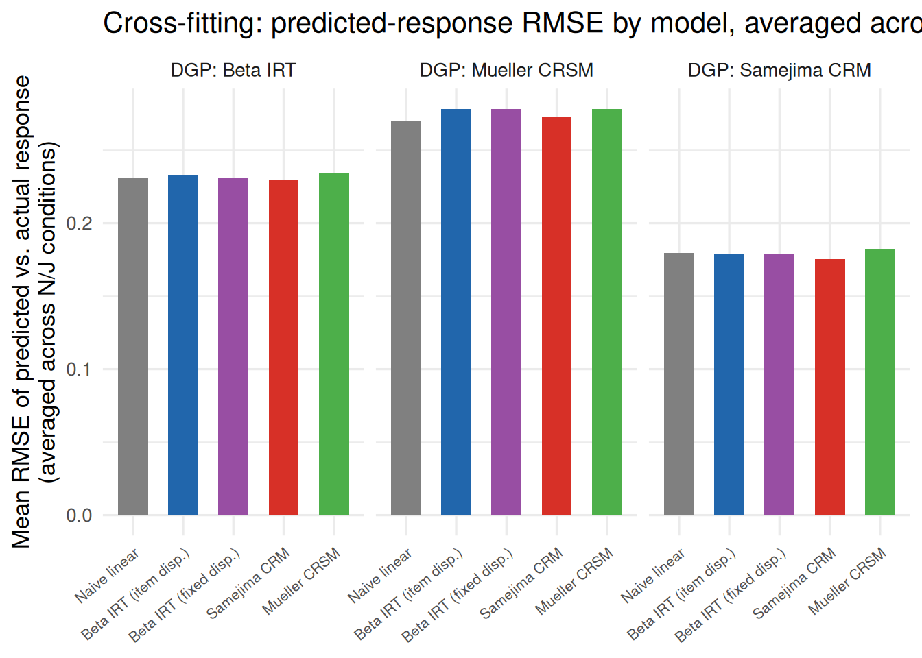
Held-out log-probability answers “how much probability mass did the model put on the interval the true response landed in” – a distributional question. It doesn’t directly answer the more concrete question the site’s binary-response vignettes usually lead with (e.g. the asymmetric IRT vignette’s predicted-vs-actual convention): if you had to guess the actual missing value, how close would you get? So alongside every log-probability number above, each model’s fitted parameters and estimated theta also produce a genuine point prediction for the same held-out cells – \(E[X_{ij}\mid \theta_i]\), the closed-form or numerically-integrated mean derived in Model equations for each spec – compared directly to the actual masked value via RMSE and correlation. The same rmse_pred/cor_pred metrics were computed for every condition in the full recovery grid above:

Code
if (grid_cache_ok) {
  grid_res$scores |>
    filter(!boundary_inflation) |>
    mutate(model = factor(model, levels = names(model_colors)),
           dgp_label = recode(dgp, beta_irt = "DGP: Beta IRT", samejima_crm = "DGP: Samejima CRM",
                               muller_corsm = "DGP: Mueller CRSM")) |>
    group_by(dgp_label, model) |>
    summarise(rmse_pred = mean(rmse_pred, na.rm = TRUE), .groups = "drop") |>
    ggplot(aes(x = model, y = rmse_pred, fill = model)) +
    geom_col(width = 0.6) +
    scale_fill_manual(values = model_colors, labels = model_labels, guide = "none") +
    scale_x_discrete(labels = model_labels) +
    facet_wrap(~dgp_label, ncol = 3) +
    labs(x = NULL, y = "Mean RMSE of predicted vs. actual response\n(averaged across N/J conditions)",
         title = "Cross-fitting: predicted-response RMSE by model, averaged across all N/J conditions per DGP") +
    theme(axis.text.x = element_text(angle = 40, hjust = 1, size = 8))
} else {
  cat("Grid cache not found -- run continuous_bounded_compute.R first.")
}
Figure 5

Where the log-probability cross-fit chart showed real (if small) separation between the 3 bounded-response models and a large, consistent gap to naive linear, RMSE shows almost none of that: all 5 specs land within about 0.01 of each other under every DGP (e.g. under the Beta IRT DGP, everything is within \([0.217, 0.222]\); under Samejima CRM’s own DGP, within \([0.176, 0.182]\)). Naive linear is never the worst of the 5 on this metric, and under Mueller CRSM’s own DGP it’s actually the numerically best (0.270 vs. Mueller CRSM’s own 0.278). Point-prediction accuracy simply isn’t where these 4 specs differ; distributional fit is – the same disconnect shows up again on real data, below.

Boundary inflation degrades RMSE for every spec by a roughly similar amount too (Beta IRT DGP, \(N=300\)/\(J=8\): naive linear 0.229 \(\to\) 0.359, the 3 bounded-response models 0.229-0.235 \(\to\) 0.351-0.378) – unlike the log-probability version of this comparison, there’s no clear asymmetry where naive linear degrades disproportionately more. That asymmetry was a distributional-fit story (a Gaussian’s tails handle boundary piling worse than the other 3 models’ densities do); it doesn’t show up in a metric that only scores the point estimate.

Summary

  • Parameter recovery works. Every correctly-specified model recovered its true item-difficulty parameters cleanly across all 16 non-inflation grid conditions (\(r>0.96\), mostly \(r>0.99\)) – the fitting code itself is sound.
  • On distributional fit (held-out log-probability), the 3 bounded-response models beat naive linear consistently, regardless of which of the 3 generated the data, and are close to interchangeable with each other: “correctly specified wins” holds only weakly, and under the Mueller CRSM DGP it doesn’t hold at all (Samejima CRM edges out Mueller’s own generating model).
  • On point predictions (RMSE), the 3 bounded-response models bring no advantage over naive linear – all 4 specs land within about 0.01 of each other under every DGP, and naive linear is never the worst. Point estimates and distributional fit are answering different questions, and only the second one is where these models actually differ.
  • Boundary inflation hurts every spec’s log-probability, but hurts naive linear roughly twice as much (~20% degradation vs. ~8-10% for the 3 bounded-response models) – none of the 4 specs has a dedicated zero-one-inflated component, so none handles it well, but the 3 bounded-response models absorb it better. RMSE shows no such asymmetry.
  • Round-number heaping (multi-modal clumping at the floor, midpoint, and quarter-points, simulated as noise independent of \(\theta\)) degrades every spec, with naive linear worst but only modestly so (~17% vs. ~12-15% for the 3 bounded-response models) – a real but much smaller gap than boundary inflation’s roughly 2x split, and one that doesn’t come close to reproducing the size of the real-data gap it was designed to test (see Real data below). What specifically closes that gap in real data – theta-correlated heaping, ceiling-dominant heaping severity, or something else – isn’t resolved here.

Taken together: under known, controlled conditions, the 3 bounded-response models do what they’re built to do – they fit the shape of a bounded response better than a model that ignores the bounds, especially once responses pile up at the boundary or heap at multiple round points at once. Whether that translates to real IRW tables, where the true generating process isn’t known and neither dial is under our control, is the question Real data below takes up next.

Real data

Simulation above established that every correctly-specified model recovers its parameters and that the 3 bounded-response models beat naive linear on held-out fit under known, controlled conditions. This section checks whether the same patterns hold on real IRW tables, where the true generating process is unknown.

Real-data selection

Candidate tables were identified by scouting IRW for tables with irw_metadata()$n_categories >= 12 whose response range and irw_tags() item-format both point to a bounded, fixed-scale response, then narrowed to tables that pass structural fitness checks for these 4 models specifically (unique (id, item) pairs – reducing to a single wave/rater where IRW’s wave/rater columns require it, no ipsative/compositional row-sum constraint, and genuine fractional-value evidence rather than a merely fine-grained integer scale). 11 tables survive and are used for every real-data result below – 7 with all 4 core specs fitting cleanly, and 4 more (added in a later pass) where one spec fails to fit for a specific, documented reason (see Limitations) but the rest of the comparison remains valid:

Table N J Note
lsbq_maleki_2025_non_persian_proficiency 308 3 0-10 scale, ~40% non-integer responses – primary evidence of genuine continuity
ai_fear_dong_2026_ai (Doctor facet, subsampled) 2,000 8 0-100, integer-valued; large-N structural check
much_tte_2025_currentmotivation 1,244 3 wave-filtered to one occasion
test_taking_much_2025_cm 1,244 9
nas_rogoza_2024_study5_nas 277 4 wave-filtered; Narcissistic Antagonism subscale
nas_rogoza_2024_study5_ngs 274 4 wave-filtered; Narcissistic Grandiosity subscale
nas_rogoza_2024_study5_nvs 278 4 wave-filtered; Narcissistic Vulnerability subscale
mendes_2019_snycq 157 12 wave-filtered; 0-100, ~27% non-integer; Samejima CRM fails to fit
westhoff2023_stopd 109 5 wave-filtered; Beta IRT fails to fit (both variants)
westhoff2023_pbat 109 18 wave-filtered; Samejima CRM fails to fit
gilbert_meta_95 115 12 wave-filtered; Beta IRT fails to fit (both variants)

ai_fear_dong_2026_ai is a 48-item, 6-target x 8-trait factorial design (Care/Doctor/Journalist/Judge/Manager/Religious x competent/warm/etc.); only one target’s 8 items (Doctor_*) are used here as a single “overall impression of Doctor” construct, not the full table.

Full scouting and per-table vetting code, cached candidate lists, and the exact reason every non-included candidate was set aside all live in vignettes/continuous_scout_* and vignettes/continuous_bounded_data/ vet_candidates*.R / vet_results*.csv – start there rather than re-deriving the logic if extending this vignette to more tables.

Real data: what do these response distributions actually look like?

Code
if (cache_ok) {
  as.data.frame(res$real$Y_raw) |>
    tidyr::pivot_longer(everything(), names_to = "item", values_to = "resp") |>
    ggplot(aes(x = resp)) +
    geom_histogram(binwidth = 0.5, boundary = 0, fill = irw_blue, color = "white", linewidth = 0.1) +
    facet_wrap(~item, ncol = 3) +
    labs(x = sprintf("Raw response (%g-%g scale)", res$real$low, res$real$high),
         y = "Count",
         title = sprintf("%s:\nraw response distribution by item", res$real$table)) +
    theme(plot.title = element_text(size = 12))
} else {
  cat("Cache not found -- run continuous_bounded_compute.R first.")
}
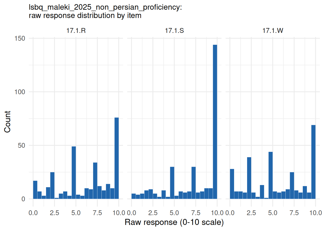
Figure 6

The primary table’s histogram above isn’t just “a hump plus a boundary spike” – look at which exact values are most common, not just the bins. For all 3 items, the top 5 response values by frequency are, in order, 10 (the ceiling), 5 (the midpoint), 7.5, 2.5, and 0 – the 5 quarter-points of the 0-10 scale, in descending order of how salient each one is as a “round number.” On item 17.1.S, that’s 44.5% of responses at exactly 10 and another 9.1% at exactly 5; combined, over half of every item’s responses land on one of these 5 points. This is response heaping: respondents (or whatever process generated these ratings) gravitating to salient round fractions of the scale, not spreading continuously across it – a well-documented phenomenon in self-report scales, here compounded by the fact that one of the 5 heap points happens to sit at the scale’s hard boundary. The result is a genuinely multi-modal response distribution, and multi-modality is a problem none of this vignette’s 4 specs is built to solve – Beta IRT, Samejima CRM, and Mueller CRSM’s conditional response densities are just as unimodal as naive linear’s Gaussian is, only bounded and more flexibly shaped.

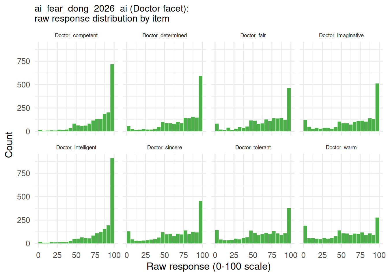
That distinction – boundary piling vs. multi-modal heaping across the whole scale – turns out to matter a lot, and a second table makes the contrast concrete. ai_fear_dong_2026_ai (Doctor facet, 0-100 scale, 8 items, \(N=2{,}000\)) also piles up near its ceiling, comparably severely on some items, but its next-most-common values are 98, 99, 97, 96, 95, 90 – a smooth decay of nearby-to-the-ceiling integers, not a separate spike at the scale’s midpoint:

Code
if (cache_ok) {
  as.data.frame(res$real2$Y_raw) |>
    tidyr::pivot_longer(everything(), names_to = "item", values_to = "resp") |>
    ggplot(aes(x = resp)) +
    geom_histogram(binwidth = 5, boundary = 0, fill = irw_green, color = "white", linewidth = 0.1) +
    facet_wrap(~item, ncol = 4) +
    labs(x = sprintf("Raw response (%g-%g scale)", res$real2$low, res$real2$high),
         y = "Count",
         title = sprintf("%s (%s facet):\nraw response distribution by item", res$real2$table, res$real2$facet)) +
    theme(plot.title = element_text(size = 12),
          strip.text = element_text(size = 7))
} else {
  cat("Cache not found -- run continuous_bounded_compute.R first.")
}
Figure 7

Counting the same top-of-scale histogram bin for both tables, lsbq’s 3 items put 22-47% of responses in the top 5% of the range (mean 31%); ai_fear_dong_2026_ai’s 8 items range 14-46% (mean 27%) – close enough that peak boundary-bin height alone doesn’t distinguish them. Despite that similarity, naive linear’s held-out log-probability is night and day between the two: -1.50 on ai_fear_dong_2026_ai, in the same range as the 3 bounded-response models (-1.18 to -1.31), against lsbq’s catastrophic -6.08 (see Held-out fit across all 11 real tables below). Multi-modal heaping, present on lsbq and absent on ai_fear_dong_2026_ai, is the most obvious candidate explanation, but it’s a hypothesis, not a demonstrated mechanism: the Simulation section’s response-heaping condition, built specifically to test it, only reproduces a small fraction of this gap. Something about real heaping – its correlation with \(\theta\), its concentration at the ceiling specifically, or some combination – matters in a way the simulated version doesn’t fully capture; see that section for the actual numbers and what was tried.

Held-out fit across all 11 real tables

Code
if (cache_ok) {
  all_real_scores <- dplyr::bind_rows(
    res$real$scores |> dplyr::mutate(N = res$real$N, J = res$real$J),
    res$real2$scores |> dplyr::mutate(
      N = res$real2$N, J = res$real2$J,
      label = paste0(label, " (", res$real2$facet, ")")
    ),
    res$batch$scores
  )
}

# One row per model, one point per table on that model's row -- lets you
# hover a point to see which table/condition it is, rather than reading
# facet titles across a grid of small bar charts.
make_strip_plot <- function(df, value_col, x_lab, title_txt) {
  df <- df |>
    dplyr::mutate(
      model = factor(model, levels = names(model_colors)),
      model_label = factor(model_labels[as.character(model)],
                            levels = rev(model_labels[names(model_colors)])),
      tbl_label = sprintf("%s (N=%d, J=%d)", label, N, J),
      value = .data[[value_col]]
    )
  # title is set via plotly::layout() below, not ggplot's own labs(title=...):
  # ggplotly() converting a ggplot title into a plotly annotation was
  # clipping the text at the plot edge. The modebar (camera/zoom icon row)
  # is disabled below too -- at narrower viewport widths it overlaps the
  # right end of a long title, obscuring the last word or two; these are
  # simple exploratory charts that don't need pan/zoom/export controls.
  p <- ggplot(df, aes(x = value, y = model_label, color = model,
                       text = sprintf("%s<br>%s: %.3f", tbl_label, x_lab, value))) +
    geom_point(size = 2, alpha = 0.85,
               position = position_jitter(height = 0.1, width = 0, seed = 1)) +
    scale_color_manual(values = model_colors, guide = "none") +
    labs(x = x_lab, y = NULL)
  plotly::ggplotly(p, tooltip = "text", height = 300) |>
    plotly::layout(
      title = list(text = title_txt, x = 0.02, xanchor = "left", font = list(size = 14)),
      margin = list(t = 45, l = 150, r = 20, b = 45),
      hoverlabel = list(align = "left")
    ) |>
    plotly::config(displayModeBar = FALSE)
}
Code
if (cache_ok) {
  make_strip_plot(all_real_scores, "mean_ll",
                   "Mean held-out log-probability (per response)",
                   "Held-out fit by model, across all 11 real IRW tables analyzed")
} else {
  cat("Cache not found -- run continuous_bounded_compute.R first.")
}
Figure 8

Each row above is one model; each point is one of the 11 real tables – hover a point for the table name and exact value. The pattern is consistent across all 11 tables and matches the simulation results above:

  • The naive linear baseline is clearly worst everywhere it’s compared, often by a wide margin – e.g. on the primary lsbq_maleki_2025_non_persian_proficiency table, naive linear’s mean held-out log-probability is -6.08, against -1.13 to -2.51 for the 3 bounded-response models. Peak boundary-bin height alone doesn’t explain the gap: ai_fear_dong_2026_ai has comparably severe peak ceiling piling on some items yet naive linear scores -1.50 there, close to the 3 bounded-response models’ own range. Multi-modal heaping – lsbq also has a secondary spike at the scale midpoint, ai_fear_dong_2026_ai doesn’t – is the leading candidate explanation (see the distribution comparison above), though a simulation built to test it only partially confirms it.
  • Among the 7 tables where all 3 bounded specs fit successfully, Samejima CRM is the worst of the 3 on every single one – sometimes by a wide margin (lsbq: -2.51 vs. -1.13 to -1.51 for the other two), sometimes narrowly (ai_fear_dong_2026_ai: -1.31 vs. -1.18).
  • Beta IRT (either dispersion variant, interchangeably) wins outright on 6 of the 11 tables: lsbq, ai_fear_dong_2026_ai, much_tte_2025_currentmotivation, test_taking_much_2025_cm, mendes_2019_snycq, and westhoff2023_pbat – the last 2 are tables where Samejima CRM wasn’t fit at all, see below.
  • Mueller CRSM wins the 3 narcissism subscales from nas_rogoza_2024_study5 (nas/ngs/nvs).
  • Samejima CRM’s only 2 wins (gilbert_meta_95, westhoff2023_stopd) are both tables where Beta IRT itself failed to fit – among tables where all 3 bounded specs were actually in the running, Samejima never wins. One plausible reason: its held-out score depends on an empirically-estimated residual SD on the transformed \(Z\) scale (see .crm_resid_sd() in continuous_bounded_helpers.R, chosen because EstCRM’s own EM-shrinkage precision term isn’t straightforward to reverse-engineer), which may generalize to genuinely new items less well than the other 2 specs’ fitted dispersion parameters do – a real cost of the workaround, not asserted with certainty.

Each table has only one train/test split (see Limitations). The main takeaway holds regardless of which of the 3 wins: all 3 bounded-response models consistently and substantially beat the naive linear baseline across every real table analyzed, on genuinely held-out item responses.

Predicted responses in real data: point estimates, not just probabilities

As in Simulation above, held-out log-probability only answers “how much probability mass did the model put on the interval the true response landed in” – a distributional question, not the more concrete “if you had to guess the actual missing value, how close would you get?” So alongside every log-probability number above, each model’s fitted parameters and estimated theta also produce a genuine point prediction for the same held-out cells – \(E[X_{ij}\mid\theta_i]\), the closed-form or numerically-integrated mean derived in Model equations for each spec – compared directly to the actual masked value via RMSE and correlation.

Code
if (cache_ok) {
  make_strip_plot(all_real_scores, "rmse_pred",
                   "RMSE of predicted vs. actual response (held-out)",
                   "Predicted-response accuracy by model, across all 11 real IRW tables")
} else {
  cat("Cache not found -- run continuous_bounded_compute.R first.")
}
Figure 9

Same layout as above – one row per model, one point per table, hoverable. This is where the story genuinely changes:

  • Naive linear’s point predictions are competitive with, and often better than, all 3 bounded-response models – the opposite of the log-probability picture. It has the lowest RMSE of all specs it’s compared against on 7 of the 11 tables: much_tte_2025_currentmotivation (0.0999), test_taking_much_2025_cm (0.1048), nas_rogoza_2024_study5_ngs (0.1799), westhoff2023_stopd (0.1684), westhoff2023_pbat (0.1970, vs. Beta IRT’s 0.3302 – a large gap in naive’s favor on that table specifically), mendes_2019_snycq (0.2666), and, most strikingly, the primary lsbq_maleki_2025_non_persian_proficiency table (0.2238, ahead of Samejima CRM’s 0.2331, Beta IRT’s 0.2459/0.2498, and Mueller’s 0.2680).
  • That’s despite naive linear having by far the worst log-probability everywhere, including a catastrophic -6.08 on lsbq against -1.13 to -2.51 for the 3 bounded-response models on that same table.
  • It’s essentially tied for best on ai_fear_dong_2026_ai (0.1961 vs. Beta IRT’s 0.1958), and only clearly beaten on 3 of the 11 (nas and nvs, by Mueller CRSM and Beta IRT respectively; gilbert_meta_95, by Samejima CRM).

This isn’t a contradiction – it’s what the two metrics are built to catch. RMSE only checks whether the central tendency is right; log-probability also checks the shape of the distribution around it (tail behavior, non-constant variance near the boundaries, how much mass piles up at 0 and 1). A linear model’s conditional mean can be a perfectly reasonable guess at where a response will land even while its Gaussian, constant-variance error structure is badly wrong about how confident to be near a boundary – exactly the boundary and midpoint heaping shown in the histograms above. So: if the applied question is “predict this person’s missing response as a single number,” the extra machinery of a bounded-response model buys little to nothing here. If the applied question involves uncertainty – uses fitted probabilities, is calibration-sensitive, or the response sits near a boundary and getting the shape right actually matters – the naive baseline’s advantage disappears entirely and the 3 bounded models are the clear right choice.

Code
if (cache_ok) {
  res$real$predictions |>
    mutate(model = factor(model, levels = names(model_colors))) |>
    ggplot(aes(x = actual, y = predicted, color = model)) +
    geom_abline(slope = 1, intercept = 0, linetype = "dashed", color = "grey50") +
    geom_point(alpha = 0.6, size = 1.6) +
    scale_color_manual(values = model_colors, labels = model_labels, guide = "none") +
    facet_wrap(~model, ncol = 3, labeller = as_labeller(model_labels)) +
    coord_equal(xlim = c(0, 1), ylim = c(0, 1)) +
    labs(x = "Actual (held-out) response", y = "Predicted response",
         title = sprintf("Predicted vs. actual held-out response:\n%s", res$real$table)) +
    theme(plot.title = element_text(size = 12),
          panel.spacing = unit(1.4, "lines"))
} else {
  cat("Cache not found -- run continuous_bounded_compute.R first.")
}
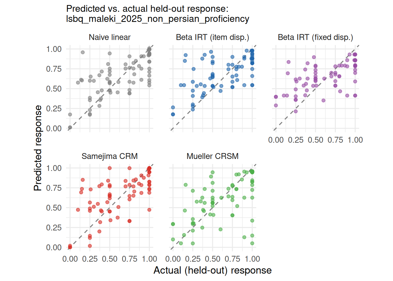
Figure 10

The scatter for the primary table makes the RMSE numbers concrete: all 5 specs track the dashed 45-degree line reasonably well across the middle of the range, and none of them is dramatically better calibrated to the point values themselves than the others – the real differentiator among models in this vignette is the log-probability metric, not this one. That’s just one table, though – the strip plot below shows the same predicted-vs-actual correlation (cor_pred) for every model on every one of the 11 real tables, the same layout as the RMSE and log-probability strip plots above:

Code
if (cache_ok) {
  make_strip_plot(all_real_scores, "cor_pred",
                   "Correlation of predicted vs. actual response (held-out)",
                   "Predicted-response correlation by model, across all 11 real IRW tables")
} else {
  cat("Cache not found -- run continuous_bounded_compute.R first.")
}
Figure 11

Same story as the RMSE strip plot: all 5 specs land in a broadly overlapping band on this metric, with no consistent separation between the 3 bounded-response models and naive linear the way there is on log-probability. Naive linear isn’t even reliably the worst here – consistent with the point-prediction metrics simply not being where these models differentiate themselves.

The same rmse_pred/cor_pred metrics were computed for every condition in the full recovery grid in the Simulation section above, including under boundary inflation – the same disconnect between RMSE/correlation and log-probability held up there too: naive linear was competitive or better on point predictions despite its consistently worse log-probability.

Summary

  • The 3 bounded-response models consistently and substantially beat naive linear on held-out log-probability, on every one of the 11 real tables – the simulation’s central finding holds up on real data, not just under known, controlled conditions.
  • Among the 3 bounded-response models, no single one dominates. Beta IRT wins outright on 6 of 11 tables, Mueller CRSM wins the 3 narcissism subscales, and Samejima CRM – worst of the 3 whenever all 3 are actually in the running – only “wins” on the 2 tables where Beta IRT itself failed to fit. As in simulation, these 3 are more interchangeable with each other than any of them is with naive linear.
  • How much worse naive linear does varies enormously by table, and tracks response heaping more than boundary piling alone. lsbq’s catastrophic -6.08 and ai_fear_dong_2026_ai’s mild -1.50 have comparably severe peak boundary piling; the difference is lsbq’s extra multi-modal heaping at the scale midpoint. Simulation’s response-heaping condition, built to test exactly this, only partially reproduces it – a real, named, still-open question this vignette raises but doesn’t close.
  • On point-prediction metrics (RMSE and correlation), naive linear is competitive with, and sometimes better than, all 3 bounded-response models – the reverse of the log-probability picture, and consistent with the same disconnect found in simulation. If the applied question needs calibrated uncertainty, the 3 bounded-response models are the clear choice; if it’s just a point guess, the extra machinery buys little here.
  • 2 of the 4 specs fail to fit outright on some real tables, for specific, diagnosed reasons (Samejima CRM’s EM on 2 tables, Beta IRT’s category-compaction issue on 2 different tables) – documented in Limitations below, not silently routed around.

Limitations

Known gaps this vignette does not yet address:

  • Ferrando’s (2001) nonlinear congeneric model (Ferrando 2001) – the optional stretch spec, comparable to the treatment in Ferrando
    1. (Ferrando 2002) – has not been attempted at all. Specs 1-4 are now complete and validated (the grid ran cleanly), so its own sequencing rule no longer blocks it – it just hasn’t been picked up yet.
  • Partial missingness in real data. All 11 real tables used complete cases only before the evaluation design’s own synthetic masking is applied; IRW tables whose respondents have naturally-occurring partial missingness (as opposed to the missingness this vignette introduces on purpose, for evaluation) aren’t handled yet.
  • The 25% per-person item-masking fraction (MASK_FRAC) was not varied or sensitivity-tested – a different fraction could shift how much information theta estimation has to work with, and thus the absolute (though probably not the relative, across-model) held-out numbers above.
  • Only one train/test split per condition (real or simulated), not a repeated/cross-validated design – so none of the held-out numbers above have an uncertainty band, and a single unlucky split could shift a close call between the 3 bounded-response models.
  • Samejima CRM’s EM is prone to failing outright, not just fitting poorly. One grid condition (Mueller-CRSM-generated, \(N=300\), \(J=8\), no boundary inflation) hit missing value where TRUE/FALSE needed during EM. This isn’t a one-off: the identical error recurred on 2 of the 4 real tables added in the follow-up vetting pass, westhoff2023_pbat and mendes_2019_snycq – both otherwise clean, wave-filtered, structurally valid tables (see Real-data selection). None of these were re-run with a different seed or diagnosed further; reported as a real, recurring misspecification/convergence fragility in EstCRM’s EM rather than something to route around.
  • Beta IRT fitting fails outright on some real tables, for a specific, confirmed reason. westhoff2023_stopd and gilbert_meta_95 (both dispersion variants) fail with response.pattern input contains more response categories than defined by the modelmirt compacts each training split’s observed categories to consecutive integers per item, and a held-out person whose response lands in a category the training split never populated gets rejected outright rather than scored as missing. This is the same failure mode described just below (originally found and fixed for a different table during development); it simply wasn’t fixable for these 2 by lowering the bin count the way it was elsewhere. Confirmed by actually running fit_score_all() on both tables (2026-08-01), not asserted from an earlier, untested claim.
  • The grid’s boundary-inflation condition covers only 1 of the 3 DGPs (Beta IRT, \(N=300\)/\(J=8\)) – not repeated for Samejima CRM or Mueller CoRSM, or at other N/J combinations.
  • Potential extension: the BoundIRT R package (Molenaar, CRAN, July
    1. fits Beta IRT, Samejima IRT, Simplex IRT, and Normal IRT under one Bayesian (Stan/MCMC) framework, which would let the held-out comparison above be replaced with a principled fully-marginalized log-likelihood (bridge sampling) or LOOIC/WAIC – a direct fix for the ad hoc bin-probability metric flagged just below – and it natively models zero/one inflation (Molenaar et al.’s (2022) extension (Molenaar et al. 2022)), which none of the 4 specs here handle despite the boundary piling documented above. It does not implement Mueller’s CRSM, so that spec would still need the current pcIRT-based code, and MCMC fitting is considerably slower than the current MLE/EM approach across 11 real tables and a 17-condition simulation grid. Not attempted here; worth a small pilot (refit Beta IRT
    • Samejima on the primary lsbq table and compare) before a full rewrite.

Package-availability and correctness issues found while building this (worth knowing before extending this vignette):

  • pcIRT::CRSM() (Mueller’s model) was dropped from the package entirely in the last CRAN release (0.2.4, 2019); it only exists in pcIRT \(\leq\) 0.2.3. pcIRT itself was later archived by CRAN entirely (2025-11-11). This vignette’s compute script installs 0.2.3 from the CRAN archive, not the current CRAN release – a real risk for reproducing this vignette in the future if the archive changes.
  • That same version’s CRSM() has a convergence-check bug (is.na(para) || ... where para becomes a 2-vector after the first iteration) that is a hard error under R \(\geq\) 4.3 and had to be patched locally before it would run at all.
  • sirt::brm.sim() hardcodes a 9-item assumption in its column-naming code and errors for any other item count; sim_beta_irt() in the helpers file reimplements its generative logic directly rather than patching sirt.
  • pcIRT::person_par.CRSM() only scores the same persons used in the original fit and has no new-data argument, so it could not be reused for scoring held-out test persons; a generalized version of its estimating equation was written from scratch instead (theta_new_muller_corsm() below) – this turned out to be a genuine improvement over the original, since it also skips NA items per person, which is exactly what made cell-level missing-response prediction possible for this spec.
  • The from-scratch Mueller CRSM person-scoring routine (theta_new_muller_corsm()) could diverge to a theta extreme enough to overflow exp() inside integrate(), which throws a hard “non-finite function value” error rather than the graceful NA stop.on.error=FALSE is supposed to allow – this crashed the entire held-out scoring pass for a table (not just Mueller CRSM) before being caught and fixed by clamping theta and wrapping each integrate() call individually.
  • Similarly, a Beta IRT scoring-stage failure (mirt compacts a training split’s observed categories to consecutive integers per item, and rejects a held-out response that lands in a category with zero training-split observations) was originally written so it could crash naive-linear/Samejima/Mueller’s results for the same table too – every model’s fit-and-score block is now wrapped in its own tryCatch so one model’s failure can’t take down the other 3.
  • The current 11 real tables are not necessarily the full set of viable candidates. See the vetting scripts/CSVs referenced in Real-data selection for the working record of what’s been checked so far.

Explicitly out of scope (not implemented, not planned for this vignette): DIF for continuous responses (Finch 2023); dual-range slider / interval-response models and the Interval Consensus Model (Kloft et al. 2024, 2023, 2025) – a different response format (an interval, not a point) and, for the Consensus Model, a different modeling paradigm (cultural consensus theory) entirely; Zopluoglu’s mixture CRM (Zopluoglu 2020) and Noel’s beta unfolding model (Noël 2014) – each adds a full second axis of complexity (latent mixture classes; unfolding vs. dominance response process), and unfolding in particular is a more natural extension of the site’s existing unfolding-vs-dominance vignette than a duplicate here; Ferrando and Navarro-Gonzalez’s (2021) multidimensional Dual Thurstonian model (Ferrando and Navarro-González 2021).

The comparison metric (held-out log-likelihood) is an ad hoc choice, not a validated best-practice for this setting – flagged explicitly above, worth revisiting.

Reproducibility

# 1. Run the compute script (from the project root)
source("vignettes/continuous_bounded_compute.R")

# 2. Re-render this page
quarto::quarto_render("vignettes/continuous_bounded.qmd")
Tip

To cite the real-data table used here, run:

irw_save_bibtex("lsbq_maleki_2025_non_persian_proficiency",
                 output_file = "continuous_bounded_data/irw_references.bib")

References

Ferrando, Pere J. 2001. “A Nonlinear Congeneric Model for Continuous Item Responses.” British Journal of Mathematical and Statistical Psychology 54 (2): 293–313. https://doi.org/10.1348/000711001159573.
Ferrando, Pere J. 2002. “Theoretical and Empirical Comparison Between Two Models for Continuous Item Responses.” Multivariate Behavioral Research 37 (4): 521–42.
Ferrando, Pere J., and David Navarro-González. 2021. “A Multidimensional Item Response Theory Model for Continuous and Graded Responses with Error in Persons and Items.” Educational and Psychological Measurement 81 (6): 1029–53. https://doi.org/10.1177/0013164421998412.
Finch, W. Holmes. 2023. “The Impact and Detection of Uniform Differential Item Functioning for Continuous Item Response Models.” Educational and Psychological Measurement 83 (5): 929–52. https://doi.org/10.1177/00131644221111993.
Kloft, Matthias, Bettina S. Siepe, and Daniel W. Heck. 2023. “The Dirichlet Dual Response Model: An Item Response Model for Continuous Bounded Interval Responses.” Psychometrika, ahead of print. https://doi.org/10.1007/s11336-023-09924-7.
Kloft, Matthias, Bettina S. Siepe, and Daniel W. Heck. 2024. “Measuring the Variability of Personality Traits with Interval Responses: Psychometric Properties of the Dual-Range Slider Response Format.” Behavior Research Methods, ahead of print. https://doi.org/10.3758/s13428-024-02394-4.
Kloft, Matthias, Bettina S. Siepe, and Daniel W. Heck. 2025. “The Interval Consensus Model: Aggregating Continuous Bounded Interval Responses.” Psychometrika.
Molenaar, Dylan, Mariana Cúri, and Jorge L. Bazán. 2022. “Zero and One Inflated Item Response Theory Models for Bounded Continuous Data.” Journal of Educational and Behavioral Statistics 47 (6): 693–735. https://doi.org/10.3102/10769986221108455.
Müller, Helmut. 1987. “A Rasch Model for Continuous Ratings.” Psychometrika 52 (2): 165–81. https://doi.org/10.1007/BF02294232.
Noël, Yvonnick. 2014. “A Beta Unfolding Model for Continuous Bounded Responses.” Psychometrika 79: 647–74. https://doi.org/10.1007/s11336-013-9361-1.
Noël, Yvonnick, and Bruno Dauvier. 2007. “A Beta Item Response Model for Continuous Bounded Responses.” Applied Psychological Measurement 31 (1): 47–73. https://doi.org/10.1177/0146621605287691.
Samejima, Fumiko. 1973. “Homogeneous Case of the Continuous Response Model.” Psychometrika 38 (2): 203–19. https://doi.org/10.1007/BF02291114.
Verhelst, Norman D. 2019. “Exponential Family Models for Continuous Responses.” In Theoretical and Practical Advances in Computer-Based Educational Measurement, edited by Bernard P. Veldkamp and Cor Sluijter. Springer.
Zopluoglu, Cengiz. 2020. “A Finite Mixture Item Response Theory Model for Continuous Measurement Outcomes.” Educational and Psychological Measurement, ahead of print. https://doi.org/10.1177/0013164419856663.