Asymmetric IRT Models Across IRW: Do LPE, RH, and AO Beat the 2PL?
Shim & Bonifay (2026) introduce three IRT models with asymmetric item response functions – LPE, RH, and AO – and show, via simplex-sampled synthetic data, that two of them fit about as well as a standard 2PL even when fitting propensity alone is compared, while the third (RH) is more parsimonious. They never apply the models to real data. We do: after a dedicated correctness/recovery validation gate, we fit a 2PL reference plus all three asymmetric models across dozens of binary IRW tables and score every model on genuinely held-out responses (InterModel Vigorish, not in-sample BIC). The two metrics tell very different stories: RH looks like the dominant winner by BIC, but is the weakest of the three – often the worst model in the batch – once judged on real predictive accuracy.
Published
October 23, 2026
Note
This vignette — including the model implementation, the validation gate, the dataset search, the compute script, and the writing below — was produced largely by Claude (Anthropic), working from a task specification and with human review. The custom item types used here are a non-trivial extension of mirt; treat the methodological choices and results accordingly, and check asymmetric_irt_helpers.R and the validation gate directly if you’re relying on the numbers shown.
Explore the model shapes
The three asymmetric models below are easier to feel than to read as equations. Pick one, drag \(\kappa\), and watch the fitted curve (blue) pull away from the symmetric baseline it’s compared against everywhere in this vignette (grey dashed) — the standard logistic 2PL for LPE and AO, a normal-ogive model for RH.
Background
Every IRT model used elsewhere on this site — the 2PL, the graded response model, the Dutch Identity’s loglinear framework — has a symmetric item response function: the probability of a correct or endorsing response rises smoothly and symmetrically around the item’s difficulty. But nothing requires that. A guessing-prone multiple-choice item, for instance, has a response curve that rises quickly from a nonzero floor and then flattens gradually near the top — asymmetric around its inflection point.
Shim and Bonifay (2026) study three such asymmetric models, each adding a single shape parameter \(\kappa\) to a standard two-parameter item:
LPE (Logistic Positive Exponent): \(P(\theta) = [\Psi(z)]^{\kappa}\), where \(\Psi\) is the logistic CDF and \(z = a(\theta - b)\). Raising the logistic curve to a power skews it toward one tail.
RH (Residual Heteroscedasticity): \(P(\theta) =
\Phi\!\left(z / \sigma(\theta)\right)\), where \(\sigma(\theta) = \sqrt{2}\,
[1 + \exp(-\kappa\theta)]^{-1/2}\) and \(\Phi\) is the normal (probit) CDF. Here asymmetry comes from letting the response variance itself change with \(\theta\), rather than from a power transform.
AO (Aranda-Ordaz, after the link function’s origin, (1981)): \(P(\theta) = 1 - [1 + \kappa\exp(z)]^{-1/\kappa}\).
In all three, a symmetric baseline is a special case: \(\kappa = 1\) recovers the ordinary logistic 2PL for LPE and AO, and \(\kappa = 0\) recovers a 2-parameter normal-ogive model for RH. The paper’s own contribution is methodological, not empirical: using synthetic data sampled arbitrarily from the response-probability simplex (not generated from any of these models), they show LPE and AO have fitting propensity statistically indistinguishable from the 2PLM — so any real advantage isn’t just an artifact of the extra parameter — while RH is more parsimonious, fitting arbitrary data somewhat less readily. They never fit any of the three models to real item response data.
That’s the gap this vignette fills: do LPE, RH, and AO actually improve on a standard 2PL across real IRW instruments, and — since Shim & Bonifay frame asymmetry around phenomena like guessing (a leniency effect concentrated at the low end of \(\theta\)) — does the direction of the fitted asymmetry relate to construct_type, e.g. more leniency in cognitive/educational items than in opinion/attitude items?
Implementing three custom, hand-derived item types is the highest-risk part of any vignette on this site, so before touching a single real IRW table we ran a dedicated validation gate — shown next — and only proceeded to the real data once it passed.
Validation: does the implementation actually behave correctly?
Each model type was implemented as a custom mirt item, with the paper’s own \(P\)/\(dP\)/\(d^2P\) math (copied, not re-derived) cross-checked against the authors’ own reference implementation. Three checks had to pass before any real IRW table was fit.
(a) Symmetric-baseline reduction
At \(\kappa = 1\) (LPE, AO) or \(\kappa = 0\) (RH), each custom item’s \(P(\theta)\) should exactly reproduce its symmetric reference model.
Table 1: Maximum absolute difference between each custom item’s P(theta) at its symmetric baseline and the corresponding reference model, evaluated on a 401-point theta grid from -6 to 6.
Model
Reference
Max |diff|
Pass
AO
2PLM (logistic)
1.11e-16
TRUE
LPE
2PLM (logistic)
1.11e-16
TRUE
RH
2-parameter normal-ogive (probit)
1.11e-16
TRUE
All three differences are at machine precision (1.1e-16 or smaller) — the custom items reduce to their reference models exactly, not just approximately.
(b) LPE non-crossing property
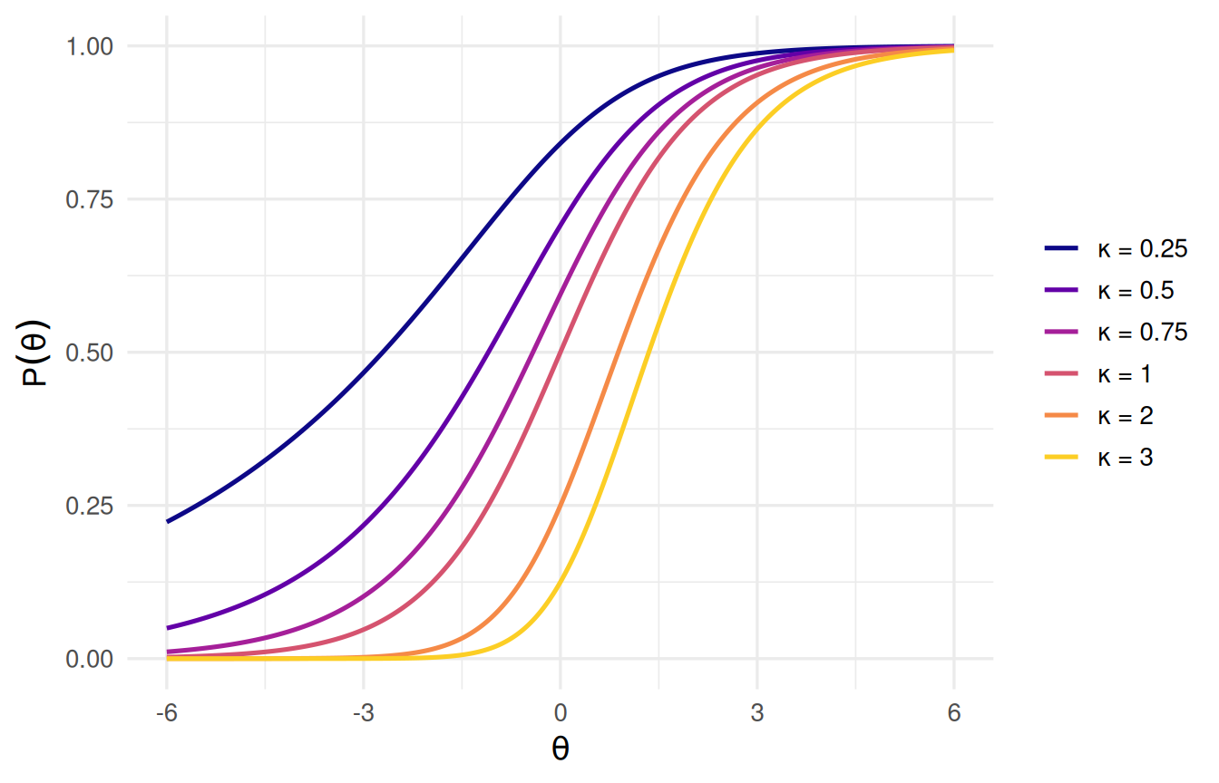
Shim and Bonifay (2026) (Section 2.1) prove that LPE curves at different \(\kappa\) never cross: for \(\kappa < 1\) the curve sits at or above the \(\kappa = 1\) curve at every \(\theta\), and for \(\kappa > 1\) it sits at or below it. This is a strong, cheap check directly on the \(P\) function.
Figure 1: LPE item response curves at six values of kappa (a = 1, d = 0). Curves for kappa < 1 sit at or above the kappa = 1 curve everywhere; curves for kappa > 1 sit at or below it. No crossing is visible anywhere on the grid.
Non-crossing holds across every pair of \(\kappa\) values checked (0.25, 0.5, 0.75, 1, 2, 3): TRUE.
(c) Simulation recovery
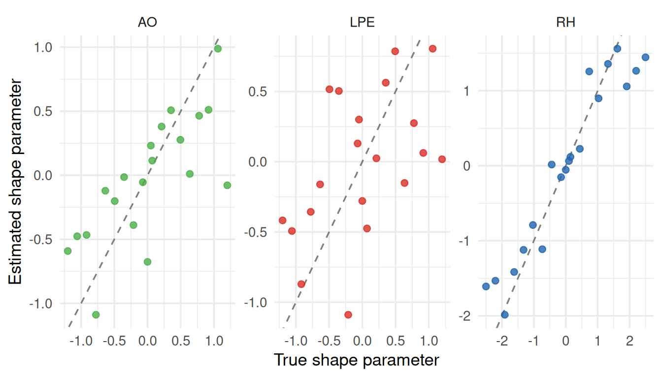
Finally, we simulated data from each model at known, clearly asymmetric \(\kappa\) values (\(N = 2{,}000\) persons, 20 items — matching the real-data scale used below) and fit the corresponding custom item to see whether the true shape parameter comes back out.
Figure 2: Shape-parameter recovery: true vs. estimated kappa (natural, unconstrained estimation scale) for each model, N = 2,000 simulated persons, 20 items. The dashed line is exact recovery.
Table 2: Correlation and mean absolute error between true and estimated shape parameters, by model.
Model
Correlation
Mean abs. error
AO
0.742
0.371
LPE
0.509
0.534
RH
0.958
0.352
Recovery is strong for RH (\(r = 0.96\)), moderate for AO (\(r = 0.74\)), and weakest for LPE (\(r = 0.51\)) — though clearly better than noise. This check draws only a single simulated dataset per model (20 items each), so these correlations are themselves noisy estimates of each model’s true recoverability at this sample size — LPE’s correlation in particular shouldn’t be read as a precise number, just as “visibly weaker than RH.” Checks (a) and (b) above involve no simulation or optimization and pass at machine precision on every machine we’ve tried; the out-of-sample calibration check in (d) below passes cleanly; and check (e) below sweeps sample size with multiple replicates per cell, giving a more precise picture of how much noise to expect at this scale than this single-dataset check can. Treat LPE’s per-item \(\kappa\) estimates below with the most caution as a result, RH’s with the least, and AO’s in between. The real-data batch below still uses a higher participant floor (\(N \geq
2,000\)) than other IRW vignettes for the same underlying reason: shape parameters are harder to pin down than location/discrimination.
(d) Out-of-sample predictive check: does BIC actually predict genuine improvement?
The real-data comparison below scores every model on held-out responses (response-level holdout, not k-fold — a fixed ~20% of each table’s observed cells are masked before fitting, then compared against predictions), using the InterModel Vigorish [IMV; Domingue et al. (2025)] rather than in-sample BIC. Before trusting that pipeline at batch scale, we ran it on synthetic data where the truth is known: does it behave sensibly when there’s genuinely no asymmetry to find, and does an in-sample BIC preference reliably translate into a held-out predictive edge?
Raw IMV values are hard to eyeball without a reference scale, so throughout the Results section below we anchor them against the benchmark ladder in Domingue et al. (2024), which reports both simulation-based and empirical (89 real dichotomous-item datasets, several drawn from the IRW) IMV values for a sequence of familiar IRT modeling upgrades: item-mean → 1PL is large (IMV ≈ 0.1–0.3), 1PL → 2PL is an order of magnitude smaller (IMV ≈ 0.006–0.01), and 2PL → 3PL — adding one extra item parameter, structurally the closest published comparison to adding a single shape parameter to a 2PL as LPE/RH/AO do here — is smaller still (simulation: 0.0005; empirical average across their 89 datasets: 0.00016, max 0.0046). That last row is the natural yardstick for the numbers below.
Table 3: Out-of-sample IMV (each asymmetric model vs. a 2PLM reference, on held-out cells) under a genuinely symmetric truth and under known, realistic-magnitude asymmetry. Five simulated replicates per cell; positive means the asymmetric model predicts better.
Under a genuinely symmetric truth, mean held-out IMV sits close to zero for all three models (confirmed: \(|{\rm mean\ IMV}| < 0.01\)) — the holdout/prediction pipeline itself isn’t biased toward finding an advantage that isn’t there. But under a known, realistic-magnitude asymmetric truth, held-out IMV was not reliably positive — RH in particular showed a small negative mean IMV even when the data-generating process really was asymmetric, despite a large in-sample BIC preference for RH in the same simulations (500 to 1,500+ BIC points, depending on the run). We confirmed this wasn’t a computation bug by manually reconstructing each model’s log-likelihood from the same extract.item()/probtrace() calls used for held-out prediction and checking it matched the model’s own reported in-sample fit direction — it did. The extra shape parameter can add enough person-ability-estimation noise to offset its true signal at realistic sample sizes, even when that signal is real.
That finding is the reason this vignette scores the real-data batch below by held-out IMV rather than BIC. It also means the result shouldn’t be surprising: if a large in-sample BIC advantage for RH doesn’t reliably survive this same check on synthetic data with a known asymmetric truth, there’s no reason to expect it to survive on real IRW tables either.
All four checks passed (July 21, 2026); only then did we move to real IRW data.
(e) Consistency: do estimates converge as sample size grows?
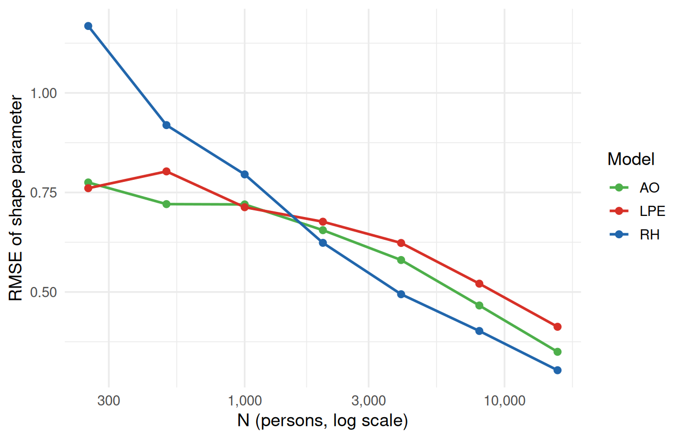
Check (c) above confirms recovery is in the right ballpark at a single sample size (\(N = 2{,}000\)) — the same scale used for the real-data batch. It says nothing about whether the estimator actually converges: whether bias and variance keep shrinking as \(N\) grows, the way a well-behaved MLE/MAP estimator should. Added as a follow-up to the original four-check gate (not a prerequisite for it — the real-data batch above was already complete when this was run), this check refits all three models across a sample-size grid from 250 to 16,000 persons, holding 12 items’ true parameters fixed throughout so that “bias at this \(N\)” is well defined, and redrawing 8 replicate person samples at every sample size.
Code
ggplot(convergence_summary, aes(x = n, y = rmse_shape, colour = model)) +geom_line(linewidth =0.9) +geom_point(size =2) +scale_x_log10(labels = scales::label_comma()) +scale_colour_manual(values = model_colors) +labs(x ="N (persons, log scale)", y ="RMSE of shape parameter", colour ="Model")
Figure 3: RMSE of the recovered shape parameter (AO: eta on the log-kappa scale; LPE: S; RH: delta) vs. sample size, one line per model. Points are averaged across items and replicates at each N; converged fits only. A consistent estimator should trend toward zero as N grows.
Table 4: Bias and RMSE of the recovered shape parameter, plus RMSE of discrimination (a) and difficulty (d), by model and sample size. Converged fits only, averaged across items and replicates.
Model
N
Fits
Bias (shape)
RMSE (shape)
RMSE (a)
RMSE (d)
AO
250
8
-0.056
0.775
0.367
0.465
AO
500
8
0.027
0.721
0.345
0.416
AO
1000
8
0.012
0.720
0.318
0.417
AO
2000
8
0.026
0.655
0.321
0.427
AO
4000
8
-0.039
0.580
0.262
0.362
AO
8000
8
-0.001
0.466
0.182
0.238
AO
16000
8
0.002
0.350
0.142
0.217
LPE
250
8
-0.012
0.761
0.757
1.670
LPE
500
8
-0.003
0.803
0.514
1.442
LPE
1000
8
-0.010
0.713
0.448
1.283
LPE
2000
8
0.000
0.677
0.334
1.107
LPE
4000
8
0.066
0.623
0.304
1.091
LPE
8000
8
0.085
0.521
0.262
0.903
LPE
16000
8
-0.011
0.413
0.180
0.650
RH
250
8
0.018
1.168
0.231
0.211
RH
500
8
-0.013
0.919
0.167
0.122
RH
1000
8
-0.013
0.795
0.112
0.088
RH
2000
8
0.048
0.623
0.079
0.065
RH
4000
8
-0.003
0.494
0.057
0.055
RH
8000
8
-0.028
0.402
0.034
0.029
RH
16000
8
-0.023
0.303
0.029
0.023
RMSE of the shape parameter falls with \(N\) for all three models — by 55% for AO ( 0.78 to 0.35), 46% for LPE ( 0.76 to 0.41), and 74% for RH ( 1.17 to 0.3), moving from the smallest to the largest \(N\) tested. The trend isn’t perfectly monotone at every step for every model — with only 8 replicates per cell there’s real sampling noise in each point in Figure 3 — but none of the three plateaus or reverses direction, which is what a consistent estimator should look like. (The raw RMSE values aren’t directly comparable across models: each model’s true shape values were drawn from a different range, matching check (c)’s convention, so a larger RMSE for one model at a given \(N\) can just as easily reflect a wider true-parameter scale as a harder estimation problem. The within-model trend across \(N\) is the finding here, not the between-model ranking.) That supports treating check (c)’s single-\(N\) recovery numbers, and the real-data batch’s per-item \(\kappa\) estimates below, as genuinely improvable with more data rather than stuck at some irreducible floor. It does not make them precise at the sample sizes IRW tables actually offer: even at the largest \(N\) tested here, shape-parameter RMSE is still several times larger than discrimination or difficulty RMSE at the same \(N\) (see Table 4) — consistent with check (c)’s finding that shape parameters are harder to pin down than location/discrimination, and the reason for this vignette’s higher-than-usual participant floor (\(N \geq 2,000\)).
NoteA closer look: what’s driving these curves, and a nuance check (c) alone doesn’t show
The improvement is a variance story, not a bias-correction one. Bias in the recovered shape parameter hovers near zero at every \(N\) tested (-0.06 to 0.09 across every model x \(N\) cell, no trend with \(N\)), so the RMSE decline in Figure 3 reflects shrinking sampling variance around an already-roughly-unbiased estimator, not a systematic offset that only shows up at small \(N\). That’s a cleaner form of consistency than a falling RMSE alone would guarantee.
LPE’s shape parameter doesn’t just recover poorly on its own — it’s entangled with \(d\).Table 4 understates this: LPE’s difficulty (\(d\)) RMSE runs 2.6–3.8\(\times\) AO’s at every sample size tested, and the gap to RH widens from 7.9\(\times\) at the smallest \(N\) to 27.8\(\times\) at the largest — not because LPE’s \(d\) estimate gets worse, but because RH’s \(d\) converges unusually fast (down to 0.023 by \(N = 16,000\)). LPE’s power-transform parameterization — raising the whole logistic curve to \(\kappa\) — couples location and shape more tightly than AO’s or RH’s link functions do. Check (c)’s “LPE recovers shape weakest” finding looks like one symptom of a broader identifiability property of the LPE parameterization, not an issue isolated to \(\kappa\) — read LPE’s per-item \(a\)/\(d\) estimates elsewhere in this vignette with that in mind, not just its \(\kappa\).
One wrinkle not to over-read. LPE’s shape-parameter RMSE ticks up slightly from \(N=250\) to \(N=500\) in Figure 3 before resuming its decline. With only 8 replicates per cell, that’s most plausibly sampling noise in which particular replicates got drawn, not a real non-monotonicity in the underlying estimator — confirming which would need more replicates per cell than this check budgeted for.
Binary items only — polytomous extensions of LPE/RH/AO are future work, not attempted here. 65 tables met this criterion as of July 2026; 57 of them produced usable results across all four models (the rest were dropped for too few usable items after cleaning, a model that failed to converge, or an irw_long2resp() limitation with a handful of tables that carry a date column).
For each candidate table, fit_asymmetric_irt():
Fetches the table and builds a wide response matrix (irw_fetch() + irw_long2resp()), capping at 10,000 respondents and canonicalizing item coding to 0/1 (IRW tables aren’t guaranteed to use 0/1 — some use 1/2 — and the held-out scoring below requires literal 0/1 outcomes).
Masks a response-level holdout: ~20% of each table’s observed cells, chosen per person so that everyone keeps at least one retained response (real IRW tables can carry substantial pre-existing missingness on top of this mask; naive cell-level masking can otherwise strand a person with zero retained responses). The same mask is reused for every model fit below, so all comparisons are on identical held-out cells.
Fits a standard 2PL as the reference model on the masked training data, on a fixed 50-point Gauss-Hermite quadrature.
Fits LPE, RH, and AO as custom items on the same masked training data, initialized from the 2PL fit (RH’s \(a\)/\(d\) are first converted from logit to probit scale) and regularized toward the symmetric baseline with a \(N(0, 1)\) prior on each shape parameter — the paper’s “moderate shrinkage” condition. Each fit is wrapped in tryCatch; non-convergent fits are logged and dropped rather than retried.
For each fitted model, estimates each person’s ability from their retained (non-masked) responses only (fscores(..., method = "EAP")), then predicts the held-out cells from that model’s own item parameters (extract.item() + probtrace()). Compares each asymmetric model’s held-out predictions against the 2PL reference’s via imv::imv.binary(), and records the winning model by IMV.
Extracts, per item, the shape parameter \(\kappa\) and \(\text{Л}_P\) (paper Eq. 7: \(\text{Л}_P = P(b+x) + P(b-x) - 1\) at \(x = 1\) logit from the item’s own difficulty \(b\)) — positive \(\text{Л}_P\) means leniency (the item is easier than a symmetric model would predict, in the sense described below), negative means strictness.
Code
fit_asymmetric_irt <-function(table_name) { resp <-fetch_wide(table_name) # irw_fetch() + irw_long2resp(), cleaned, 0/1-coded ho <-mask_holdout(resp, frac =0.2) # per-person cell mask, >=1 response retained per person fit_2pl <-mirt(ho$train, 1, itemtype ="2PL", technical =list(customTheta = Theta_mat_ref, ...)) fit_lpe <-fit_custom(ho$train, "LPE", make_custom_item("LPE"), ad_start =extract_ad(fit_2pl), ...) fit_rh <-fit_custom(ho$train, "RH", make_custom_item("RH"), ad_start =convert_ad_logit_to_probit(...), ...) fit_ao <-fit_custom(ho$train, "AO", make_custom_item("AO"), ad_start =extract_ad(fit_2pl), ...)# theta from retained responses only, predictions on held-out cells, IMV vs. the 2PL reference th_2pl <-fscores(fit_2pl, method ="EAP") p_2pl_heldout <-heldout_preds(fit_2pl, th_2pl, ho$mask_idx)# ... same for LPE/RH/AO, then imv::imv.binary(ho$true_vals, p_2pl_heldout, p_model_heldout) ...}
Note
To reproduce with current IRW holdings, re-run validation_gate.R then asymmetric_irt_compute.R, and commit the updated asymmetric_irt_data/asymmetric_irt_results.rds.
Table 5: Winning model by out-of-sample IMV, across all tables with usable results.
Winning model
# Tables
%
2PLM
23
40.4
LPE
15
26.3
AO
12
21.1
RH
7
12.3
The plain 2PLM wins outright in the largest share of tables. Among the asymmetric models, RH — the model that looked dominant by BIC — wins the least often, behind both LPE and AO. That’s a striking reversal from what in-sample BIC would suggest, and it’s exactly the pattern the validation-gate synthetic check above warned to expect: a large in-sample BIC edge for RH doesn’t reliably survive contact with genuinely held-out data.
Figure 4: Best asymmetric-model out-of-sample IMV relative to the 2PL reference, one point per table, ranked from most-improved to least. Positive values favor the asymmetric model; color shows which model achieved that best IMV (2PLM = no asymmetric model improved on it). Hover for details.
There’s no long dramatic tail in Figure 4 the way there was for BIC: IMV values cluster close to zero on both sides, and even the largest positive values are modest by IMV standards — well under 0.01, and in the same neighborhood as Domingue et al. (2024)’s empirical IMV(2PL,3PL) benchmark (average 0.00016, max 0.0046 across their 89 datasets), not their IMV(1PL,2PL) benchmark (average ≈ 0.006–0.01). That places the predictive value of these asymmetric shape parameters alongside one of the weakest published IRT modeling upgrades, not a meaningful one — a world away from the BIC deltas running into the hundreds of points for the same tables. Whatever asymmetric structure is real in these data, its predictive value is small.
Table 6: Winning model by construct_type (multi-tagged combinations collapsed into the first matching bucket).
Construct bucket
AO
LPE
RH
2PLM
Cognitive/educational
5
5
2
0
Opinion/attitude
6
7
2
18
Other
1
2
1
1
Unknown
0
1
2
4
Construct type is far more diagnostic here than it was under BIC (where RH won in every bucket regardless). Among Cognitive/educational tables, the plain 2PLM never wins — some asymmetric model always predicts at least marginally better out of sample. Opinion/attitude tables show the opposite pattern: 2PLM wins the clear majority. That split is a real, substantive finding in its own right, separate from the leniency-direction question below.
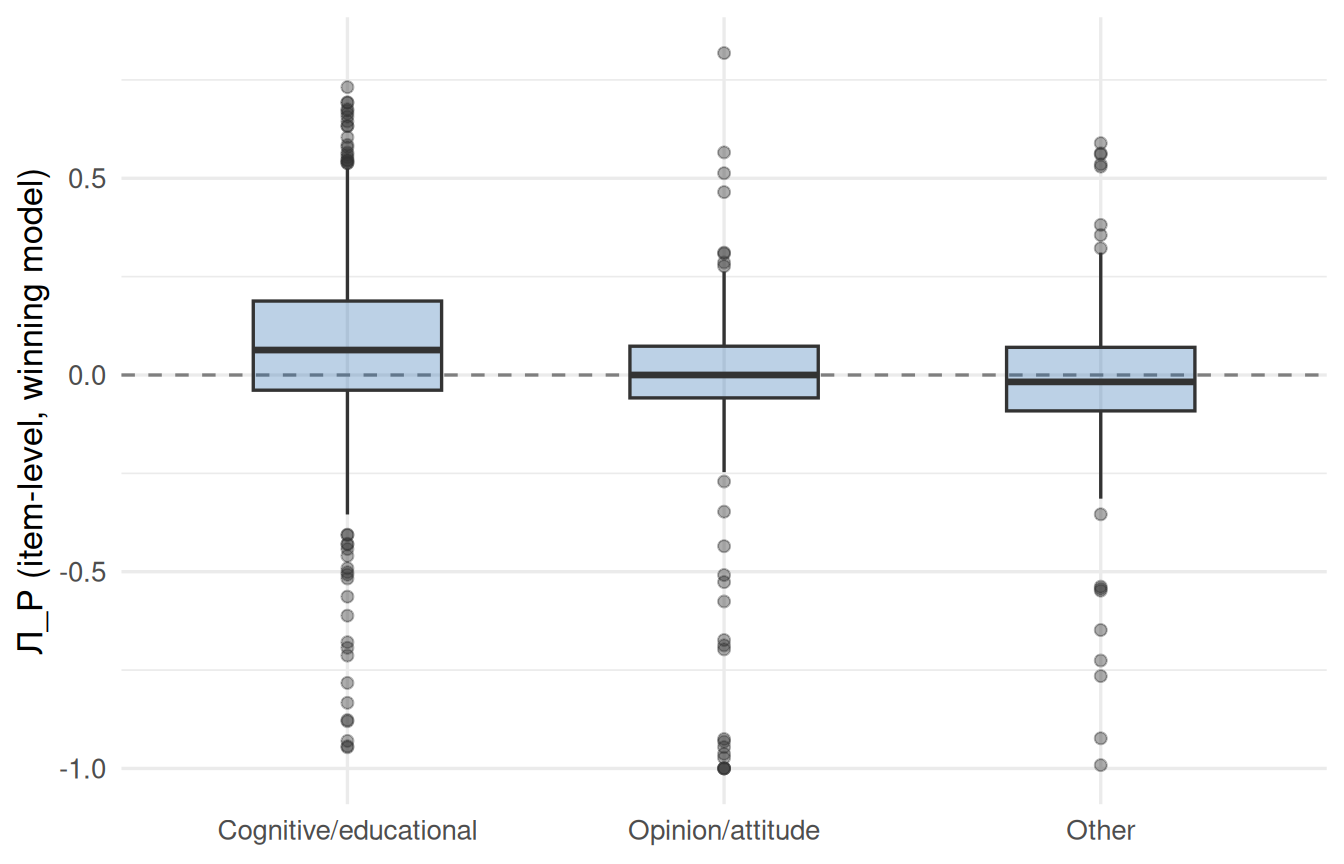
Figure 5: Distribution of item-level Л_P (positive = leniency, negative = strictness) for the winning model’s items in each table, by construct bucket. Dashed line at zero.
Cognitive/educational items skew toward leniency (mean \(\text{Л}_P\) = 0.069, 67% of items positive) while Opinion/attitude items skew the other way, toward strictness (mean \(\text{Л}_P\) = -0.039, only 51% positive). That’s a full sign flip between construct types, not just a difference in degree — a cleaner separation than the same comparison showed under the old BIC-based winning model, and squarely the direction the guessing hypothesis predicts (guessing on cognitive items should show up as leniency at the low end of \(\theta\)). Both buckets still have items on either side of zero, so treat this as a real, directionally consistent pattern rather than a hard rule at the individual-item level.
One example of a genuine (if modest) win
colombia_2023_politics_attitudes has the single largest positive out-of-sample IMV in this batch (LPE beats the 2PL by 7.90e-03 on held-out responses). That’s still comfortably under Domingue et al. (2024)’s IMV(1PL,2PL) benchmark ceiling (empirical max 0.068), but it’s roughly on par with their average IMV(1PL,2PL) (0.006) — i.e., this single best case in the whole batch is about as valuable as a typical 1PL-to-2PL upgrade, while the typical table here (per Figure 4) sits down in IMV(2PL,3PL)-negligible territory. Its item item_p5261s7 (LPE: \(a\) = 7.45, \(b\) = 1.35, \(\kappa\) = 0.1, \(\text{Л}_P\) = 0.465) shows a substantial item-level asymmetry even though the table-level predictive gain is small — below, the fitted LPE curve is plotted against the symmetric logistic curve that the same\(a\) and \(b\) would imply under \(\kappa = 1\) (the exact reduction validated above), i.e. what a standard 2PL would have predicted for this item. Several other items in this same table show the opposite sign (strong implied strictness, \(\text{Л}_P \approx -1\)) at implausibly extreme \(\kappa\) — the thin-data outliers flagged in Limitations below, not shown here. That mix of a real, sizeable item-level effect in one direction and unreliable extreme estimates in others is exactly why the table-level aggregate win ends up modest rather than dramatic.
Figure 6: Fitted LPE item response curve (blue) vs. the symmetric logistic curve implied by the same discrimination and difficulty (grey dashed), for the item with this batch’s largest genuine out-of-sample IMV win. Orange points are empirical bins – observed endorsement rate within 10 EAP-theta groups, the same binning mirt::itemfit(…, empirical.plot=) uses internally, sized by group n. Hover to compare predicted response probabilities at any theta, or see each bin’s observed rate and n.
This item’s discrimination is unusually high (\(a\) = 7.5), which is exactly the regime where empirical theta-bins can look noisy bin-to-bin even when the underlying model fit is sound: a tiny shift in who lands in which bin, near a near-step-function response curve, swings the observed rate a lot. Read the smooth fitted curves as the main comparison here, and the empirical points as a rough check rather than a precise one for this particular item.
The LPE curve sits above the symmetric reference through most of the lower and middle trait range and only catches up near the top — exactly the qualitative signature of \(\kappa < 1\) (0.1 here) and positive \(\text{Л}_P\): a person one logit above and one logit below this item’s difficulty are, on average, more likely to endorse it than a symmetric model centered on the same difficulty would predict.
Limitations
Binary items only. LPE/RH/AO extensions to polytomous items exist in principle but weren’t attempted here.
Fixed regularization. The \(N(0,1)\) MAP prior on each shape parameter is the paper’s own “moderate shrinkage” condition, applied uniformly; no per-table prior-sensitivity sweep was run at IRW scale (the paper does run one, in a different context).
RH is probit-linked; the others are logistic. RH is not exactly nested in the logistic 2PLM the way LPE and AO are. Scoring every model by held-out IMV on the response probability scale sidesteps the specific caution the paper raises about comparing BIC across link functions — IMV only needs comparable predicted probabilities, not a comparable likelihood parameterization — but RH’s probit link is still a real, separate modeling choice from the other two, worth keeping in mind when comparing its \(\kappa\) to LPE/AO’s.
Per-item shape estimates are noisy, and a few are extreme. A handful of items — typically ones that are answered almost unanimously one way — show implausibly large \(|\kappa|\) (up to roughly 26 for AO, 52 for LPE, and -7 to 6 for RH in this batch), consistent with the imperfect recovery documented above (weakest for LPE, moderate for AO, strongest for RH) rather than a broken fit, but not individually verified case by case. Treat extreme per-item \(\kappa\) values as thin-data artifacts unless checked directly — the worked example above shows this concretely: several items in that same table hit \(\text{Л}_P \approx -1\) at extreme \(\kappa\), alongside the one genuinely interesting item featured there.
The response-level holdout is generous but not huge. ~20% of each table’s observed cells, capped so every person keeps at least one retained response — enough to detect the null-truth calibration cleanly in the validation gate, but individual held-out IMV values for smaller tables (some under 2,500 respondents) are based on proportionally fewer held-out cells than the largest tables and should be read with that in mind.
Shape-parameter recovery is imperfect and uneven across models. See the discussion in Validation (c) above — RH recovers well (\(r = 0.96\)), AO moderately (\(r = 0.74\)), and LPE weakest (\(r = 0.51\)). Treat LPE’s per-item \(\kappa\) with the most caution, RH’s with the least.
A shape parameter may be structurally hard to identify at all, not just noisy to estimate.(Holland 1990)’s conservation law — worked out in detail in this site’s Dutch Identity vignette — shows that a unidimensional test of \(J\) items supports at most \(2J\) parameters as \(J \to \infty\), exactly the 2PL’s \((a, d)\) budget per item; the 3PL’s third parameter (guessing) exceeds that budget, and that vignette finds empirically that the 2PL → 3PL predictive gain shrinks toward zero as test length grows. LPE, RH, and AO are in the same structural position: each adds one third per-item parameter (\(\kappa\)) on top of an otherwise-2PL base, mechanically identical to how the 3PL adds guessing. That framing fits two things found here better than “these models just need more data”: the real-data IMV gains above sit at the IMV(2PL,3PL) benchmark rather than the substantially larger IMV(1PL,2PL) one, and the sample-size sweep in check (e) found LPE’s shape parameter doesn’t fail cleanly on its own — it drags its own difficulty (\(d\)) estimate down with it, exactly the kind of budget-overrun a third per-item parameter would produce if a unidimensional test’s real information ceiling is the two the 2PL already spends. This isn’t the same asymptotic Holland’s theorem uses (that result is about test length \(J \to \infty\) with \(N\) effectively unlimited; check (e) is about sample size \(N \to \infty\) with \(J\) fixed at 12 items) — so treat it as a motivating frame for why\(\kappa\) is hard to pin down, not as a confirmation of the conservation law itself.
These results were computed against approximately IRW v265 (the corpus as of July 23, 2026).
NoteHow this version was determined
The version was inferred from when the results were computed, not recorded during the run, so it may be off by a version or more. This version pins one or more IRW shards to a release whose own date Redivis lost in a platform migration, so which release of those shards was live that day is reconstructed rather than recorded. To pin data to an exact version, use irw_use_version().
Results were computed on July 21, 2026. To regenerate:
# 1. Re-run the validation gate (from the project root)source("vignettes/asymmetric_irt_data/validation_gate.R")# 2. Re-run the real-data batchsource("vignettes/asymmetric_irt_compute.R")# 3. Re-fit the single worked example and extract its empirical theta binssource("vignettes/asymmetric_irt_data/example_itemfit_compute.R")# 4. Re-run the sample-size convergence sweep (validation gate check (e))source("vignettes/asymmetric_irt_data/convergence_sim_compute.R")# 5. Re-render this pagequarto::quarto_render("vignettes/asymmetric_irt.qmd")
Aranda-Ordaz, F. J. 1981. “On Two Families of Transformations and Goodness of Fit.”Biometrika 68 (2): 357–63.
Domingue, Benjamin W., Klint Kanopka, Radhika Kapoor, et al. 2024. “The InterModel Vigorish as a Lens for Understanding (and Quantifying) the Value of Item Response Models for Dichotomously Coded Items.”Psychometrika 89 (3): 1034–54. https://doi.org/10.1007/s11336-024-09977-2.
Domingue, Benjamin W., Charles Rahal, Jessica Faul, et al. 2025. “The InterModel Vigorish (IMV) as a Flexible and Portable Approach for Quantifying Predictive Accuracy with Binary Outcomes.”PLOS ONE 20 (3): e0316491.
Holland, Paul W. 1990. “The Dutch Identity: A New Tool for the Study of Item Response Models.”Psychometrika 55 (1): 5–18. https://doi.org/10.1007/BF02294739.
Shim, Hyejin, and Wes Bonifay. 2026. “On the Asymmetry, Complexity and Predicted Data Patterns of Nontraditional Item Response Theory Models.”British Journal of Mathematical and Statistical Psychology, ahead of print. https://doi.org/10.1111/bmsp.70069.