Dimensionality Across IRW: How Often Does Unidimensionality Hold?

Every unidimensional IRT model used elsewhere on this site – 1PL, 2PL, the IMV comparisons – assumes item responses are explained by a single latent trait. We compute item correlation matrices for every eligible IRW table and run two classic exploratory diagnostics, the eigenvalue ratio and parallel analysis, to see how often that assumption actually holds and whether it varies by construct type.

Note

This vignette — including the dataset search, the compute script, the analysis design, and the writing below — was produced largely by Claude (Anthropic), working from a task specification and with human review. Treat the methodological choices and interpretations accordingly, and check the compute script (dimensionality_compute.R) directly if you’re relying on the numbers here.

Motivation

Every unidimensional IRT model used elsewhere on this site — the 2PL fits across cognitive datasets, the IMV comparisons, the Dutch Identity — rests on the same starting assumption: a single latent trait explains the pattern of item correlations. That assumption is a convenience as much as a claim about the world. Real instruments often bundle related but distinct sub-facets (a “self-regulation” battery with attention, inhibition, and working-memory items), or are built explicitly as multi-factor scales (a personality inventory with five named traits). Fitting a 1PL/2PL to multidimensional data doesn’t produce an error — it produces a single composite ability estimate that quietly averages over whatever structure was actually there. This vignette asks a simple empirical question: across real IRW instruments, how often does the data actually look one-dimensional, and does that vary by construct type? It then asks the complement — what happens when several instruments given to the same respondents are merged back into one battery — since a single IRW table is usually a single instrument, which caps how multidimensional any one table can be.

We use two classic exploratory diagnostics, not a confirmatory test: the ratio of the first to second eigenvalue of the item correlation matrix (larger = more consistent with one dominant factor), and parallel analysis (Horn 1965) — comparing the observed eigenvalues to those expected from random data. Both flag candidates for multidimensionality; neither tells you what the extra dimensions are or whether they’re substantively meaningful. The CFA vignette shows the confirmatory next step for any table flagged here.

Data and methods

Dataset selection

all_candidates <- irw_filter(
  n_items        = c(5, 40),
  n_participants = c(200, Inf)
)

We cap items at 40 (and require at least 5) for compute reasons: tetrachoric and polychoric correlation matrices, and parallel analysis on top of them, both scale poorly as item count grows, and this needs to run across every eligible IRW table. 913 tables met this criterion as of July 2026. The cap also bounds how multidimensional anything in this pass can look; the merged-battery section relaxes it to 150 items for a smaller, curated set of multi-instrument studies. This pass analyzes all 913 of them.

Per-table computation

For each candidate table, fit_dimensionality():

1. Fetches the table and builds a wide response matrix (irw_fetch() + irw_long2resp()), downsampling to at most 10,000 respondents and dropping zero-variance items, mirroring the 2PL across datasets and local dependence pipelines.
2. Builds an item correlation matrix appropriate to the response type: tetrachoric (psych::tetrachoric()) for binary items, polychoric (psych::polychoric()) for 3-10 response categories, and a Pearson fallback (logged explicitly) for anything outside that range — mostly continuous slider items, which show up as tables with a large number of distinct response values.
3. Eigen-decomposes the correlation matrix and records the ratio of the 1st to 2nd eigenvalue and the proportion of total variance the 1st eigenvalue explains.
4. Runs parallel analysis (psych::fa.parallel(), factor extraction, no plot) against a simulated random-data baseline, recording the suggested number of factors. Wrapped in tryCatch — this can fail on small or ill-conditioned matrices, in which case the table is logged and dropped rather than crashing the batch.
5. Records, per table: item/respondent counts, correlation method used, eigenvalue ratio, proportion of variance on factor 1, parallel-analysis suggested factor count, plus construct_type and item_format from IRW’s tags for the breakdown below.

fit_dimensionality <- function(table_name) {
  resp   <- fetch_wide(table_name)  # irw_fetch() + irw_long2resp(), cleaned
  cormat <- if (n_categories == 2) tetrachoric(resp)$rho
            else if (n_categories <= 10) polychoric(resp, max.cat = 10)$rho
            else cor(resp, use = "pairwise.complete.obs")
  ev <- eigen(cormat, symmetric = TRUE, only.values = TRUE)$values
  pa <- fa.parallel(cormat, n.obs = nrow(resp), fa = "fa", plot = FALSE)
  # ... ratio_12 <- ev[1] / ev[2]; suggested factors <- pa$nfact ...
}

Of the 913 candidate tables in this pass, 810 produced usable results (the rest were dropped for too few usable items or a correlation/eigendecomposition that failed outright).

Note

To reproduce with current IRW holdings, re-run dimensionality_compute.R and commit the updated dimensionality_data/dimensionality_results.rds.

Results

How concentrated is the variance in one factor?

ggplot(summary_df, aes(x = pmin(ratio_12, 15))) +
  geom_histogram(bins = 40, fill = irw_blue, colour = "white") +
  geom_vline(xintercept = ratio_cutoff, linetype = "dashed", colour = irw_red) +
  labs(x = "1st / 2nd eigenvalue ratio (capped at 15 for display)", y = "Number of tables")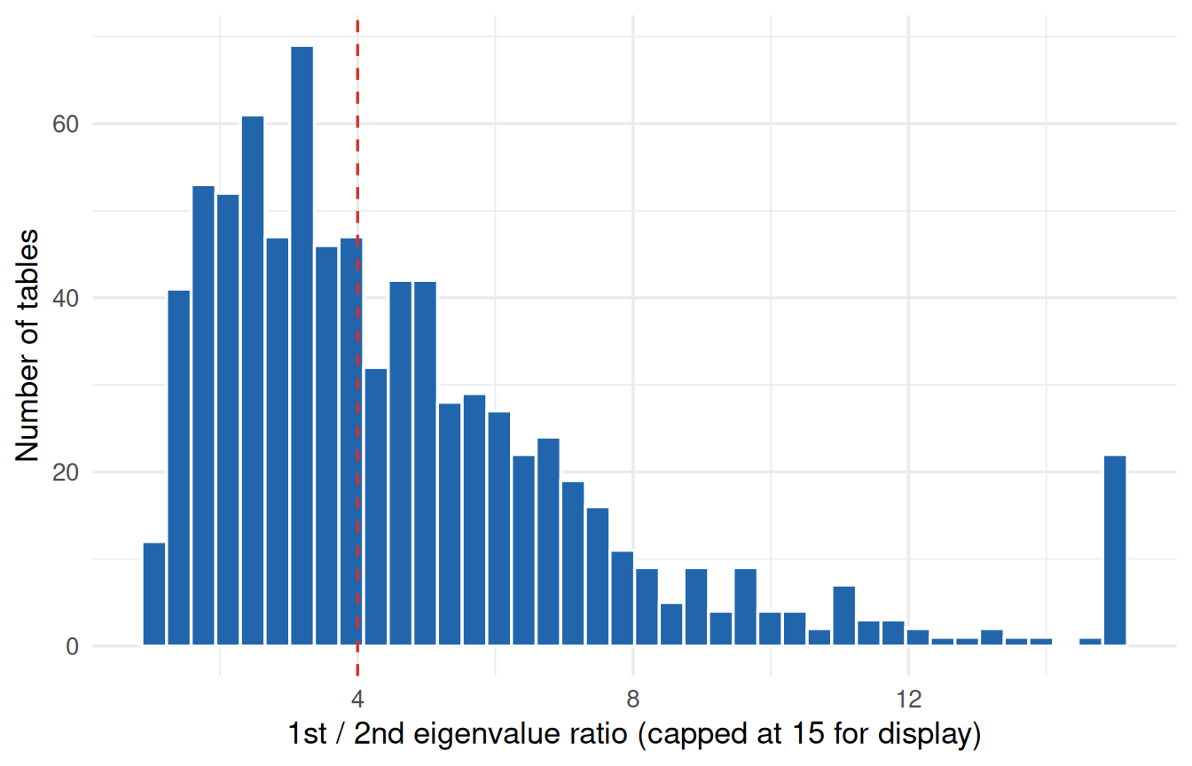

Figure 1: Ratio of the 1st to 2nd eigenvalue of the item correlation matrix, one table per bar. The dashed line marks a ratio of 4, near the top of the ~3-to-1-or-greater range sometimes read as a rough sign of approximate unidimensionality (Embretson and Reise 2000) – treat it as a rule of thumb, not a hard rule.

49% of tables (396 of 810) clear the ratio > 4 heuristic in Figure 1. Parallel analysis is much stricter: only 3% of tables (28) get a suggested factor count of exactly 1. That gap between the two diagnostics is itself the most interesting finding here — see below.

Does it vary by construct type?

construct_order <- summary_df %>%
  filter(!is.na(construct_type)) %>%
  group_by(construct_type) %>%
  summarise(med = median(ratio_12), .groups = "drop") %>%
  arrange(med) %>%
  pull(construct_type)

plot_df <- summary_df %>%
  filter(!is.na(construct_type)) %>%
  mutate(
    construct_type = factor(construct_type, levels = construct_order),
    tooltip = paste0(
      "Table: ", table,
      "<br>Ratio: ", round(ratio_12, 2),
      "<br>PA factors: ", nfact_suggested,
      "<br>n_items: ", n_items,
      "<br>Construct: ", construct_type
    )
  )

medians_df <- plot_df %>%
  group_by(construct_type) %>%
  summarise(med = median(ratio_12), .groups = "drop") %>%
  mutate(tooltip = paste0("Median (", construct_type, "): ", round(med, 2)))

p <- ggplot(plot_df, aes(x = pmin(ratio_12, 15), y = construct_type, text = tooltip)) +
  geom_jitter(height = 0.15, colour = irw_blue, alpha = 0.5, size = 1.7) +
  geom_point(data = medians_df, aes(x = pmin(med, 15), y = construct_type, text = tooltip),
             shape = 18, size = 4, colour = irw_red) +
  labs(x = "1st / 2nd eigenvalue ratio (capped at 15 for display)", y = NULL)

ggplotly(p, tooltip = "text")

Figure 2: Eigenvalue ratio by construct_type (primary label, for tables tagged with more than one). Each point is one table; diamonds mark the median within each type. Hover over a point to see which table it is.

summary_df %>%
  filter(!is.na(construct_type)) %>%
  group_by(construct_type) %>%
  summarise(
    n_tables            = n(),
    median_ratio         = median(ratio_12),
    prop_ratio_above_cut = mean(ratio_12 > ratio_cutoff),
    median_nfact         = median(nfact_suggested, na.rm = TRUE),
    .groups = "drop"
  ) %>%
  arrange(desc(median_ratio)) %>%
  knitr::kable(digits = 2, col.names = c("Construct type", "N tables", "Median ratio",
                                          "Prop. ratio > cutoff", "Median PA factors"))

Table 1: Eigenvalue ratio and parallel-analysis factor counts by construct_type (primary label).

Construct type	N tables	Median ratio	Prop. ratio > cutoff	Median PA factors
Affective/mental health	101	5.12	0.63	3.0
Physical health/functioning	7	5.06	0.86	7.0
Other	4	4.50	0.50	5.5
Cognitive/educational	141	3.74	0.43	5.0
Opinion/attitude	176	3.72	0.46	4.0
Behavioral	53	3.48	0.40	4.0
Personality	57	3.26	0.40	4.0
Developmental	9	2.55	0.22	4.0

Read Figure 2 and Table 1 together: constructs built as a single narrow skill or trait tend to sit toward the high-ratio end, while constructs assembled from several named sub-facets (a multi-scale personality or psychopathology battery folded into one IRW table) tend to sit lower. Neither diagnostic is a clean binary split — there’s substantial within-type spread — but the ranking across types is informative on its own.

Every table, ranked

ranked_df <- summary_df %>%
  arrange(ratio_12) %>%
  mutate(
    rank    = row_number(),
    tooltip = paste0(
      "Table: ", table,
      "<br>Ratio: ", round(ratio_12, 2),
      "<br>PA factors: ", nfact_suggested,
      "<br>n_items: ", n_items,
      "<br>Construct: ", construct_type
    )
  )

p <- ggplot(ranked_df, aes(x = pmin(ratio_12, 15), y = rank, text = tooltip)) +
  geom_point(colour = irw_blue, size = 1.6, alpha = 0.7) +
  geom_vline(xintercept = ratio_cutoff, linetype = "dashed", colour = irw_red) +
  labs(x = "1st / 2nd eigenvalue ratio (capped at 15 for display)", y = NULL) +
  theme(axis.text.y = element_blank(), axis.ticks.y = element_blank())

ggplotly(p, tooltip = "text") |>
  layout(margin = list(t = 60))

Figure 3: Every table’s eigenvalue ratio, ranked from lowest to highest. Hover over a point to see which table it is.

Sanity check: does the diagnostic recover a known answer?

scree_tables <- c("psychtools_bfi" = "psychtools_bfi (Big Five personality, 5 known factors)",
                   "4thgrade_math_sirt" = "4thgrade_math_sirt (single-construct math test)")

scree_df <- bind_rows(lapply(names(scree_tables), function(tbl) {
  ev <- eigenvalues_list[[tbl]]
  if (is.null(ev)) return(NULL)
  tibble(table = scree_tables[[tbl]], component = seq_along(ev), eigenvalue = ev)
}))

if (nrow(scree_df) > 0) {
  ggplot(scree_df, aes(x = component, y = eigenvalue)) +
    geom_hline(yintercept = 1, linetype = "dashed", colour = irw_grey) +
    geom_line(colour = irw_blue) +
    geom_point(colour = irw_blue) +
    facet_wrap(~table, scales = "free_x", labeller = label_wrap_gen(width = 22)) +
    labs(x = "Component", y = "Eigenvalue") +
    theme(strip.text = element_text(size = 10, lineheight = 1.1))
} else {
  cat("Sanity-check tables not present in this run.")
}

Figure 4: Scree plots for a known multi-factor personality battery (left, psychtools_bfi – 25 items, 5 named traits) and a single-construct math test (right, 4thgrade_math_sirt), for comparison. The dashed line at eigenvalue = 1 is a visual reference (the classic Kaiser criterion), not the decision rule used elsewhere in this vignette.

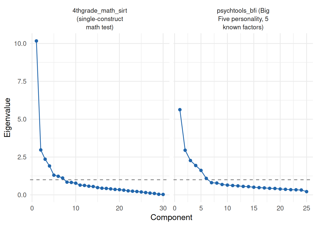
The Big Five inventory – 5 named traits by construction – has a 1st/2nd eigenvalue ratio of 1.91 and parallel analysis suggests 6 factors: both diagnostics correctly flag it as clearly multidimensional. The math test has a ratio of 3.43, well above the personality battery’s – the diagnostic moves in the expected direction even though (see below) parallel analysis alone still suggests more than one factor for it.

What happens when we merge instruments?

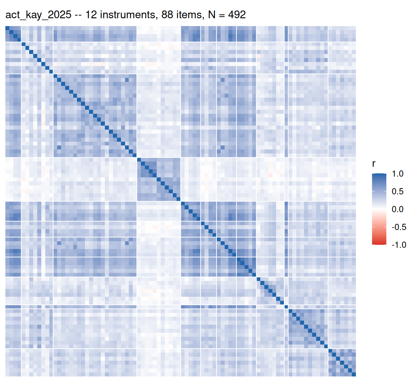
Everything above analyzes IRW tables one at a time, and that quietly caps how multidimensional the answer can be: an IRW table is usually a single instrument, so we have mostly been asking whether individual scales are internally unidimensional. The more interesting question for anyone fitting a model to a real assessment battery is what happens when a respondent’s whole session is put back together.

IRW supports exactly that. Tables sharing a DOI are typically several instruments from one study, given to one cohort, ingested separately — so stacking them recovers the full battery each respondent actually saw. The irw package exposes this directly:

# Discover and merge every table sharing a DOI (or BibTex) with this one:
merged <- irw_merge("chakraborty2026_IWAH_IRW")

irw_merge() groups by DOI (falling back to BibTex), rbinds the members, and reports consistency checks — equal N, shared respondent IDs, no item overlap — before proceeding. We don’t call it at render time for two reasons: its confirmation prompt returns its default in a non-interactive session, so those checks would pass as messages rather than filters; and a live lookup would let the figures below drift as IRW’s bibliography grows. Instead dimensionality_merge_scout.R reimplements the same grouping, applies the checks as hard filters, and freezes the survivors into dimensionality_merge_compute.R. Of 468 merge groups, 112 passed a metadata screen (3–12 member tables, identical N, 20–150 total items) and 107 survived verification against the fetched data — every member table sharing an identical respondent set with no overlapping items. Item overlap was the one substantive failure: five groups turned out to have the same instrument ingested twice under a single DOI.

Those checks are structural, though, and a group can pass all of them while still covering fewer distinct constructs than it has member tables — which would inflate the instrument-count axis in Figure 6. A further pass over member names and the construct_name field of irw_tags() removed ten groups on three grounds: one instrument split into per-subscale tables (the seven afaya_2020_*_knowledge tables are all subscales of a single diabetes-knowledge questionnaire; the seven ghanbari_2016_helma_* tables are the named subscales of HELMA); a composite scale sitting beside its own components (lorenz_2016_psycap alongside hope, efficacy, resilience and optimism); and repeated administration or duplicate ingest (okeke2025_* measures three constructs both pre and post, and one study appears under two DOIs). The exclusions and their reasons are listed in EXCLUDED_GROUPS in dimensionality_merge_compute.R, leaving 97 groups.

Each merged battery then goes through the identical pipeline used above: correlation matrix, eigen-decomposition, parallel analysis. Item names are prefixed with their source table, and the matrix is restricted to respondents present in every member table. 90 of the 97 produced usable results.

One wrinkle is specific to merging. Batteries routinely stack instruments with different scale lengths — a 5-point scale beside a 6-point one — which leaves sparse cells in the bivariate contingency tables and can drive psych::polychoric()’s default continuity correction into an unusable correlation matrix. Following psych’s own advice in that situation, those cases are retried with correct = 0, which recovered 19 batteries that would otherwise have been dropped. This doesn’t arise in the single-table pass, where one instrument means one response scale throughout.

compare_df <- bind_rows(
  transmute(summary_df, kind = "Single table", prop_var_1),
  transmute(merge_df,   kind = "Merged battery", prop_var_1)
) %>%
  mutate(kind = factor(kind, levels = c("Single table", "Merged battery")))

ggplot(compare_df, aes(x = prop_var_1, fill = kind)) +
  geom_density(alpha = 0.55, colour = NA) +
  scale_fill_manual(values = c("Single table" = irw_grey, "Merged battery" = irw_blue)) +
  labs(x = "Proportion of variance on the 1st factor", y = "Density", fill = NULL) +
  theme(legend.position = "top")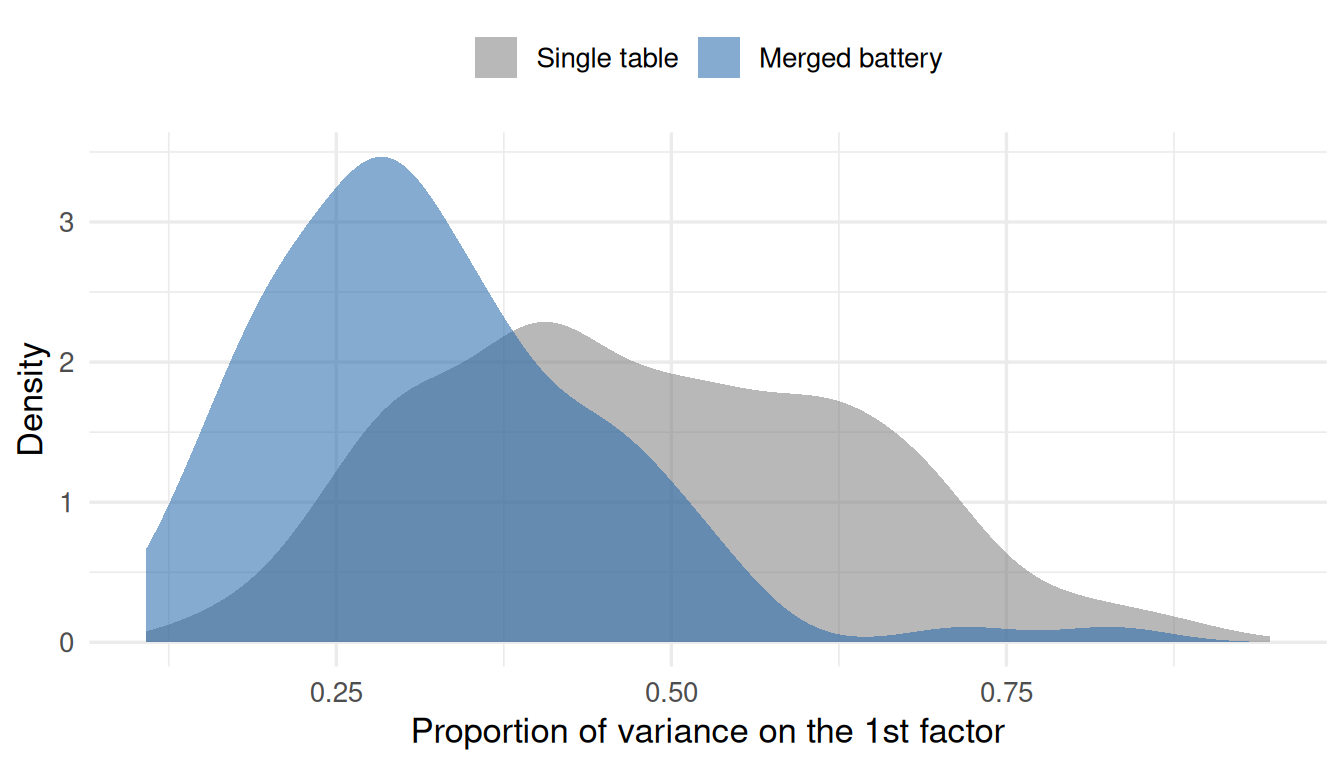

Figure 5: Proportion of item-correlation variance carried by the first factor, for single IRW tables (the analysis above) and for merged multi-instrument batteries. Merging shifts the distribution decisively downward – exactly as it should, and a useful check that the diagnostic is measuring what we think it is.

The first factor carries a median of 47% of the variance in single tables but only 30% in merged batteries, and the median eigenvalue ratio falls from 3.88 to 2.87. This is the high-dimensional end of the warehouse: real sessions in which respondents answered 3–12 distinct instruments, with a median parallel-analysis count of 7 factors.

p <- merge_df %>%
  mutate(tooltip = paste0(
    "Anchor: ", anchor,
    "<br>Instruments merged: ", n_tables,
    "<br>PA factors: ", nfact_suggested,
    "<br>Ratio: ", round(ratio_12, 2),
    "<br>n_items: ", n_items,
    "<br>N: ", n_participants
  )) %>%
  ggplot(aes(x = n_tables, y = nfact_suggested, text = tooltip)) +
  geom_abline(slope = 1, intercept = 0, linetype = "dashed", colour = irw_red) +
  geom_jitter(width = 0.15, height = 0.15, colour = irw_blue, alpha = 0.6, size = 1.8) +
  labs(x = "Number of instruments merged", y = "Parallel-analysis factor count")

ggplotly(p, tooltip = "text")

Figure 6: Parallel-analysis factor count against the number of instruments stacked into each battery. The dashed line is 1:1. Instrument count is an index of how much was merged, not a ground-truth factor count – some groups split one inventory into per-subscale tables, others repeat a construct pre/post – so read the line as a rough reference, not a target.

Two things are worth reading off Figure 6. Parallel analysis does track instrument count — merged batteries land far above the single-factor solutions common in the single-table pass — but it scatters widely around the 1:1 line rather than recovering it, and the over-extraction discussed below means points above the line are expected. Points well below the line are the more interesting ones: batteries where several nominally distinct instruments collapse into fewer empirical dimensions than the study design implies.

exemplar <- merge_df %>%
  filter(!is.na(nfact_suggested), n_items <= 150, n_tables >= 5) %>%
  filter(!sapply(anchor, function(a) is.null(merge_cormats[[a]]))) %>%
  arrange(desc(n_tables)) %>%
  slice(1)

if (nrow(exemplar) == 1) {
  cm  <- merge_cormats[[exemplar$anchor]]
  isr <- merge_items[[exemplar$anchor]]
  ord <- isr$item[order(isr$source_table, isr$item)]
  ord <- ord[ord %in% rownames(cm)]
  cm  <- cm[ord, ord]

  src      <- isr$source_table[match(ord, isr$item)]
  boundary <- which(diff(as.integer(factor(src, levels = unique(src)))) != 0) + 0.5

  hm_df <- expand.grid(row = seq_along(ord), col = seq_along(ord)) %>%
    mutate(r = as.vector(cm))

  ggplot(hm_df, aes(x = col, y = row, fill = r)) +
    geom_raster() +
    geom_vline(xintercept = boundary, colour = "white", linewidth = 0.4) +
    geom_hline(yintercept = boundary, colour = "white", linewidth = 0.4) +
    scale_fill_gradient2(low = irw_red, mid = "white", high = irw_blue,
                         midpoint = 0, limits = c(-1, 1), name = "r") +
    scale_y_reverse(expand = c(0, 0)) +
    scale_x_continuous(expand = c(0, 0)) +
    coord_fixed() +
    labs(x = NULL, y = NULL,
         subtitle = paste0(exemplar$anchor, " -- ", exemplar$n_tables,
                           " instruments, ", exemplar$n_items, " items, N = ",
                           exemplar$n_participants)) +
    theme(axis.text = element_blank(), axis.ticks = element_blank(),
          panel.grid = element_blank())
} else {
  cat("No merged battery with a cached correlation matrix in this run.")
}

Figure 7: Item correlation matrix for one merged battery, with items ordered by source instrument and white lines marking instrument boundaries. Within-instrument blocks stand out against much weaker between-instrument correlation – the structure a single eigenvalue ratio necessarily flattens into one number.

Two diagnostics, one disagreement

The eigenvalue ratio and parallel analysis agree on direction — the math test above scores more unidimensional than the personality battery on both — but they disagree sharply on the absolute call. Parallel analysis suggests exactly one factor for only 3% of tables in this sample, including tables like the math test above that most researchers would treat as reasonably unidimensional in practice. This isn’t a bug in the pipeline: it’s a documented property of parallel analysis run on tetrachoric/polychoric correlation matrices. Garrido, Abad, and Ponsoda (2013) show in a large simulation study that PA on polychoric correlations systematically over-extracts factors relative to PA on Pearson correlations, especially with few response categories, skewed items, or smaller samples — exactly the conditions common across IRW tables. The polychoric/tetrachoric correlation estimates themselves carry sampling noise that inflates later eigenvalues, and parallel analysis’s random-data baseline doesn’t fully correct for it.

Practically: treat the eigenvalue ratio in Figure 1 as the more robust of the two signals for ranking tables against each other, and treat parallel analysis’s suggested factor count as a noisy, generally inflated upper bound rather than a literal count of a table’s dimensions. A table is worth a closer confirmatory look (with the CFA vignette) when both diagnostics point the same direction — low ratio and a PA count well above 1 — rather than off either one alone.

Limitations

Exploratory, not confirmatory. Neither diagnostic tells you what the extra dimensions are, whether they’re substantively meaningful, or whether a bifactor/testlet structure (rather than several independent traits) better describes the data. The CFA vignette is the natural next step for any table flagged here.

Parallel analysis over-extracts on ordinal data, as discussed above (Garrido et al. 2013) — don’t read the suggested factor count as a literal answer to “how many dimensions does this table have.”

A single ratio collapses a lot of structure. Two tables with the same 1st/2nd eigenvalue ratio can have very different shapes underneath — one might have one dominant factor and many small residual ones, another two comparably-sized factors and nothing else. The full eigenvalue spectrum (as in the scree plots above) carries more information than the ratio alone; the ratio is used here as a single sortable number because it needs to summarize 810 tables in one figure.

Merged batteries index how much was stacked, not how many factors are really there. The number of member tables in Figure 6 counts instruments a study contributed to IRW, and IRW’s table boundaries don’t always align with construct boundaries. Groups where they clearly diverged — one inventory split into per-subscale tables, a composite beside its own components, a construct administered twice — were removed (see above), but that vetting leans on construct_name, which is populated for only about a third of the groups; the rest were judged on member names alone. Some residual construct duplication is therefore likely, and it would bias the instrument count upward, so the 1:1 line remains a reference rather than a target. Reassuringly, the comparison the section actually rests on is insensitive to this: dropping the ten clearest cases left the median first-factor variance for merged batteries unchanged (0.295) and moved the median eigenvalue ratio from 3.04 to 2.87. What the vetting changes is the credibility of the instrument-count axis, not the single-versus-merged contrast.

Local dependence and low dimensionality aren’t the same thing. A table can show local item dependence (testlets, shared stems) without failing a global dimensionality check, and vice versa. See the local dependence vignette for the complementary residual-correlation diagnostic.

Reproducibility

Source code for this page: dimensionality.qmd · dimensionality_compute.R · dimensionality_merge_compute.R · dimensionality_merge_scout.R

These results were computed against approximately IRW v301 (the corpus as of August 25, 2026).

NoteHow this version was determined

The version was inferred from when the results were computed, not recorded during the run, so it may be off by a version or more. To pin data to an exact version, use irw_use_version().

Results were computed on July 21, 2026. To regenerate:

# 1. Re-run the compute scripts (from the project root)
source("vignettes/dimensionality_compute.R")        # single-table pass
source("vignettes/dimensionality_merge_compute.R")  # merged multi-instrument batteries

# 1a. Optional: re-discover merge groups against current IRW holdings.
#     Writes candidate CSVs for review; the vetted groups are then frozen
#     into MERGE_GROUPS in dimensionality_merge_compute.R.
source("vignettes/dimensionality_merge_scout.R")

# 2. Re-render this page
quarto::quarto_render("vignettes/dimensionality.qmd")

Tip

To cite the datasets used, run:

irw_save_bibtex(summary_df$table, output_file = "dimensionality_data/references.bib")

---

References

Embretson, Susan E., and Steven P. Reise. 2000. Item Response Theory for Psychologists. Lawrence Erlbaum Associates.

Garrido, Luis Eduardo, Francisco José Abad, and Vicente Ponsoda. 2013. “A New Look at Horn’s Parallel Analysis with Ordinal Variables.” Psychological Methods 18 (4): 454–74. https://doi.org/10.1037/a0030005.

Horn, John L. 1965. “A Rationale and Test for the Number of Factors in Factor Analysis.” Psychometrika 30 (2): 179–85. https://doi.org/10.1007/BF02289447.