Latent Space Item Response Models: Seeing Local Dependence as Geometry
The Rasch model assumes local independence, but nothing about a standard fit warns you when that assumption fails. The Latent Space Item Response Model (LSIRM) adds a single respondent-item distance term and turns the same question into a picture: an “interaction map” where items and respondents that share unexplained structure are pulled close together. We fit it to 16 IRW tables – known testlet structure, suspected speededness, and blind exploratory draws – and find a split by response format so clean it forced a validity check on the estimator itself.
Published
October 23, 2026
Note
This vignette – including the dataset search, the compute script, the analysis design, and the writing below – was produced largely by Claude (Anthropic), working from a task specification and with human review. Treat the methodological choices and interpretations accordingly, and check the compute script (lsirm_interaction_maps_compute.R) directly if you’re relying on the numbers here.
Motivation
The Latent Space Item Response Model [LSIRM; Jeon et al. (2021)] adds a single extra term to the Rasch model: a distance penalty between each respondent and each item in a shared, unobserved 2D space, which lets the data decide whether local independence – the assumption that once you condition on a respondent’s position on the latent trait, their responses to different items are unrelated – actually holds. The local dependence vignette checks the same assumption a different way, with Yen’s Q3: fit the model, subtract what it predicts, and see whether anything is left to correlate between item pairs. That residual approach answers “is independence violated” with a number per pair, but it doesn’t show why items and respondents interact, or which respondents are involved. LSIRM’s distance term does both at once: when it isn’t needed, the model collapses back to an ordinary Rasch fit; when it is, respondents and items that share unexplained structure are pulled close together in the space, and the result is directly visualizable: an interaction map. Local dependence stops being an abstract residual correlation and becomes a picture – clusters you can point at.
Method in brief
For a respondent \(j\) and item \(i\) with an ordinary Rasch model, the log-odds of a correct/endorsed response would be \(\theta_j - \beta_i\) (respondent ability minus item difficulty). LSIRM adds one term:
where \(z_j\) and \(w_i\) are the respondent’s and item’s positions in a shared 2D Euclidean space, and \(\gamma \geq 0\) scales how much that distance matters. When \(\gamma = 0\), the distance term vanishes and the model is the Rasch model; the further \(z_j\) sits from \(w_i\), the more the distance term drags the predicted log-odds down relative to what \(\theta_j -
\beta_i\) alone would predict – interaction the main effects didn’t capture. Fitting the positions and \(\gamma\) jointly by MCMC produces the interaction map: a scatter of item points and respondent points in the same space, where proximity signals shared unexplained structure (a testlet, a common stimulus, a shared response tendency) rather than an ordinary ability/difficulty relationship.
Because \(\gamma = 0\) is a single point on the boundary of \(\gamma \geq 0\), it can’t be tested with an ordinary credible interval the way a normal parameter could. The package used here [lsirm12pl; Go et al. (2025)] implements the spike-and-slab model-selection extension from the original paper (Ishwaran and Rao 2005): a mixture prior on \(\log \gamma\) with a “spike” component concentrated near \(\gamma = 0\) and a “slab” component allowing \(\gamma > 0\), plus an indicator \(\phi\) for which component is active at each MCMC iteration. The posterior mean of \(\phi\) – reported below as the inclusion probability – is the model-selection answer: values near 0 mean the data are consistent with an ordinary Rasch fit; values near 1 mean the interaction term is doing real work. This resolves an open question going into this vignette (see Limitations) – the current CRAN version of lsirm12pl (2.0.3, not the 1.3.9 assumed when this vignette was scoped) exposes spike-and-slab fitting directly via lsirm1pl_ss() (dichotomous items) and lsirmgrm_ss() (graded/polytomous items), so no hand-rolled WAIC comparison was needed.
The graded-response variant is not merely a software convenience. The latent space graded response model has its own development and evaluation (De Carolis et al. 2026), which extends the binary LSIRM of Jeon et al. (2021) to ordered-category responses and is aimed squarely at the Likert-scale self-report instruments that make up most of the study set below. That matters for how the results here should be read: the polytomous fits are an application of a model developed and studied for exactly this kind of data, not an off-label use of a binary method.
Data and methods
Study-set selection
MCMC here is far more expensive per table than the mirt-based models used elsewhere on this site – the original paper’s own examples ran 30-60 minutes per table at N~200-700, I~7-24 – so this vignette deliberately selects 16 tables rather than batch-fitting across all of IRW, in two rounds:
Round 1 (hypothesis-driven, 5 tables), chosen to bracket the diagnostic:
Code
# 1. Tables with known item_family (testlet) structure -- ground truth on# which items *should* cluster if LSIRM is picking up real dependence.# Cross-referencing the local-dependence vignette's own item_family# census: only 2 of ~800 IRW tables carry a usable grouping at all.# g308_sirt is dichotomous; chakraborty2026_IWAH_IRW is graded.# 2. Tables suspected of speededness -- candidates for the "respondents# cluster near the last items" pattern described in the LSIRM paper's# discussion section. Cross-referenced against the (unmerged)# speededness-vignette branch's own classification:# credentialform_lnirt and nature_relatedness were both flagged# "likely speeded" there.# 3. A presumed-Rasch-like negative control with no known family/testlet# structure and no speededness suspicion: blum_2018_imak_bin.
Round 2 (expansion, 11 more tables), added after Round 1 cleared the go/no-go bar and raised a “what predicts a positive finding” question that needed more data points:
Code
# 4. The remaining 5 tables classified "likely speeded" by the same# speededness screen, completing that bucket in full: brain_hemisphere,# artistic_preferences, depression_anxiety_stress, fisher_temperment,# face_memory_test.# 5. A *blind* random sample (seed 20260723) of 6 more tables from# irw_filter(n_items = c(5, 60), n_participants = c(100, 5000)),# excluding every table already in the study set -- deliberately not# hand-picked for any hypothesis: sd3ypl_klimczak_2019_ses,# BPAQ_Christopher_2024_PSS10, prpt_hellmann_2021_conscientiousness,# chen2026_sc, disgust_berger2014, autism_blotner_2025_s1_aq.
Table 1: The full 16-table study set. ‘Domain’ is a rough characterization from each table’s construct/context (cognitive-ability task vs. personality/attitude/clinical self-report scale), not an IRW metadata field – flagged because it turns out to matter (see below).
table
role
domain
n_items
n_participants
n_categories
sd3ypl_klimczak_2019_ses
blind exploratory
personality/attitude/clinical
10
325
4
BPAQ_Christopher_2024_PSS10
blind exploratory
personality/attitude/clinical
10
109
5
prpt_hellmann_2021_conscientiousness
blind exploratory
personality/attitude/clinical
12
700
5
chen2026_sc
blind exploratory
personality/attitude/clinical
19
195
5
disgust_berger2014
blind exploratory
personality/attitude/clinical
25
700
5
autism_blotner_2025_s1_aq
blind exploratory
personality/attitude/clinical
40
535
4
g308_sirt
item_family
cognitive/ability
20
700
2
chakraborty2026_IWAH_IRW
item_family
personality/attitude/clinical
30
634
5
blum_2018_imak_bin
negative control
cognitive/ability
23
317
2
credentialform_lnirt
speededness suspect
cognitive/ability
40
700
2
face_memory_test
speededness suspect
cognitive/ability (graded)
40
700
5
nature_relatedness
speededness suspect
personality/attitude/clinical
32
700
8
brain_hemisphere
speededness suspect
personality/attitude/clinical
20
700
5
artistic_preferences
speededness suspect
personality/attitude/clinical
40
700
8
depression_anxiety_stress
speededness suspect
personality/attitude/clinical
40
700
8
fisher_temperment
speededness suspect
personality/attitude/clinical
40
700
8
Per-table computation
For each table, fit_lsirm() in the compute script:
Fetches the wide response matrix directly via irw_fetch(table, resp = TRUE), and separately fetches the long format to recover item_family (if present) and a within-person item-presentation-order column (same fallback logic as the speededness vignette: a named order column if one exists, first-appearance order otherwise).
Downsamples respondents to at most 700 and items to at most 40, mirroring the downsampling pattern already used in 2PL across datasets. Item downsampling always keeps the true last 10 items by presentation order (so the “stragglers near the end” check below stays meaningful) and systematically samples the rest; this triggered for every table with more than 40 items (credentialform_lnirt, depression_anxiety_stress, fisher_temperment, face_memory_test, artistic_preferences).
Fits the 1PL LSIRM with spike-and-slab (lsirm1pl_ss()) for dichotomous tables, or the graded-response variant [lsirmgrm_ss(); De Carolis et al. (2026)] for polytomous tables, both with a 2D latent space and the full 15,000-iteration MCMC settings (2,500 burn-in, thinned by 5), matching the original paper’s defaults.
Records posterior mean item and respondent positions, the \(\gamma\) posterior mean and 95% credible interval, the inclusion probability, and BIC.
To reproduce with current IRW holdings, re-run lsirm_interaction_maps_compute.R --full and commit the updated lsirmdata/lsirm_interaction_maps_results_full.rds.
Table 2: Posterior mean gamma (with 95% credible interval) and posterior inclusion probability for gamma > 0, one row per table, sorted by response format then by P(gamma > 0). Inclusion probability above 0.5 favors the latent-space model over an ordinary Rasch fit; below 0.5 favors Rasch.
Table
Format
Gamma [95% CI]
P(gamma > 0)
Model favored
prpt_hellmann_2021_conscientiousness
polytomous/graded
1.49 [1.39, 1.60]
0.997
Latent space (gamma > 0)
chakraborty2026_IWAH_IRW
polytomous/graded
1.19 [1.11, 1.27]
0.995
Latent space (gamma > 0)
sd3ypl_klimczak_2019_ses
polytomous/graded
1.26 [1.13, 1.42]
0.994
Latent space (gamma > 0)
depression_anxiety_stress
polytomous/graded
1.28 [1.23, 1.31]
0.992
Latent space (gamma > 0)
autism_blotner_2025_s1_aq
polytomous/graded
1.09 [1.03, 1.17]
0.992
Latent space (gamma > 0)
nature_relatedness
polytomous/graded
1.05 [1.01, 1.09]
0.989
Latent space (gamma > 0)
BPAQ_Christopher_2024_PSS10
polytomous/graded
0.99 [0.76, 1.20]
0.984
Latent space (gamma > 0)
face_memory_test
polytomous/graded
0.91 [0.84, 1.00]
0.983
Latent space (gamma > 0)
disgust_berger2014
polytomous/graded
0.88 [0.80, 0.96]
0.980
Latent space (gamma > 0)
chen2026_sc
polytomous/graded
0.90 [0.77, 1.06]
0.979
Latent space (gamma > 0)
fisher_temperment
polytomous/graded
0.84 [0.80, 0.92]
0.978
Latent space (gamma > 0)
brain_hemisphere
polytomous/graded
0.80 [0.75, 0.85]
0.973
Latent space (gamma > 0)
artistic_preferences
polytomous/graded
0.76 [0.72, 0.80]
0.967
Latent space (gamma > 0)
credentialform_lnirt
dichotomous
1.82 [1.53, 1.98]
1.000
Latent space (gamma > 0)
blum_2018_imak_bin
dichotomous
0.05 [0.01, 0.16]
0.012
Rasch (gamma = 0)
g308_sirt
dichotomous
0.03 [0.00, 0.08]
0.003
Rasch (gamma = 0)
In plain terms: “inclusion probability” is the model’s own confidence, on a 0-to-1 scale, that the extra “interaction” ingredient is actually needed to explain the data – above 0.5 means “yes, include it”; near 1 means “yes, almost certainly”; near 0 means “no, an ordinary Rasch model already explains this fine.” Read that way, the table above says something striking: every single one of the 13 multi-point-scale tables – including all 6 that were picked completely at random, with no reason to expect anything special – comes back with the model over 96% sure the interaction ingredient is needed. The 3 right/wrong tables split the way we originally expected going in: two come back near-certain it’s not needed (g308_sirt, blum_2018_imak_bin), and one comes back the most certain of anything in the whole set that it is needed (credentialform_lnirt, at 99.96% confidence). A split that tracks question format (right/wrong vs. multi-point scale) this cleanly – especially once random, unrelated tables were thrown in and still followed the same pattern – is a red flag worth checking before trusting it as a real finding about these tables, rather than a quirk of how the tool handles multi-point scales. That check is the next section.
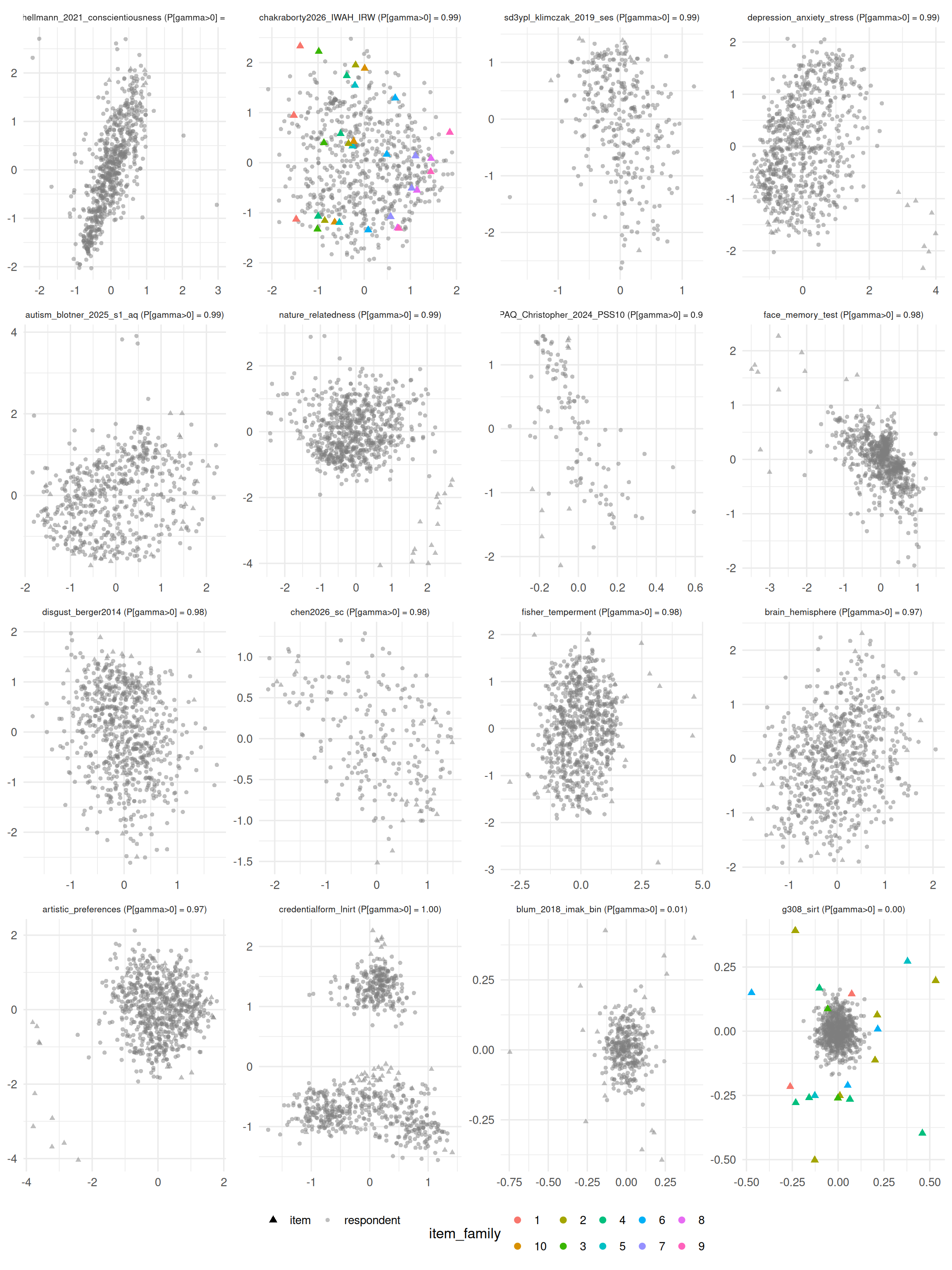
Figure 1: Interaction maps for all 16 study-set tables, grouped by response format (dichotomous first) and sorted by posterior inclusion probability within format. Points are posterior mean positions in the shared 2D latent space: circles are respondents, triangles are items. Items sharing a known item_family grouping (where available) are colored; all other points are grey. Panel titles show each table’s posterior inclusion probability for gamma > 0.
chakraborty2026_IWAH_IRW (top group, colored by item_family) shows visibly tighter item clustering by group than the two near-null dichotomous panels’ diffuse scatter. Beyond that one labeled case, though, the maps mostly demonstrate the same thing the gamma table does: broad, structured spread across nearly every polytomous panel regardless of role (speededness suspect or blind exploratory), and near-patternless noise in g308_sirt and blum_2018_imak_bin.
Is this really about response format, or is the estimator biased?
A split this clean – every multi-point-scale table positive, most right/wrong tables null – is more consistent with a quirk in the tool than with 13 independent real discoveries. Put plainly: before believing “multi-point scales have hidden structure and right/wrong tests mostly don’t,” we need to rule out the boring explanation that the fitting method itself just runs hot on any multi-point-scale data, whether or not anything real is going on. So the question gets turned on the tool: does lsirmgrm_ss() (the multi-point-scale version of the fitting method) claim high confidence on any multi-point-scale data, even data we build by hand to have zero true interaction?
Code
# Simulate a clean single-factor GRM dataset: realistic item discrimination# and category thresholds, N/I matched to the study set, gamma = 0 by# construction (no interaction structure of any kind).a <-matrix(rlnorm(20, 0, 0.3), ncol =1)d <-matrix(t(apply(matrix(rnorm(20*4), ncol =4), 1, function(x) sort(x, decreasing =TRUE))), ncol =4)sim_dat <- mirt::simdata(a, d, N =700, itemtype ="graded")sim_fit <-lsirmgrm_ss(sim_dat, ndim =2, niter =15000, nburn =2500, nthin =5)
Code
tibble(case =c("Simulated null GRM data (this check)", "Real polytomous tables (range, n=13)"),pi_estimate =c(.cache$null_calibration$pi_estimate,paste0(sprintf("%.3f", min(summary_df$pi_estimate[!summary_df$is_dichotomous]))," to ",sprintf("%.3f", max(summary_df$pi_estimate[!summary_df$is_dichotomous])))),gamma =c(sprintf("%.3f", .cache$null_calibration$gamma_mean),paste0(sprintf("%.2f", min(summary_df$gamma_mean[!summary_df$is_dichotomous]))," to ",sprintf("%.2f", max(summary_df$gamma_mean[!summary_df$is_dichotomous]))))) |> knitr::kable(col.names =c("Case", "P(gamma > 0)", "Gamma"))
Table 3: Null-calibration check: lsirmgrm_ss() fit to simulated single-factor GRM data with no true interaction structure, versus the range of results actually observed across the 13 real polytomous study-set tables.
Case
P(gamma > 0)
Gamma
Simulated null GRM data (this check)
0.0084
0.056
Real polytomous tables (range, n=13)
0.967 to 0.997
0.76 to 1.49
The tool passes this check: fed data with no true interaction at all, it correctly comes back unconfident (0.008 out of 1, essentially “no”) rather than falsely claiming there’s something there. In plain terms, that rules out the laziest explanation – the method doesn’t just rubber-stamp “yes” on every multi-point-scale dataset regardless of content – and shifts the weight of evidence toward the 13-for-13 result being a real property of these particular tables, not a broken tool. But it doesn’t fully settle the question, because of a mix-up baked into which tables happened to land in each bucket:
Response format and what the tables actually measure are tangled together here, almost perfectly. Every right/wrong table in this set is a cognitive-ability task (testlet reading comprehension, a credentialing exam, figural analogies); every multi-point-scale table (with one partial exception, face_memory_test, a graded confidence/memory task rather than a personality scale) is a Likert-type personality, attitude, or clinical self-report scale (conscientiousness, disgust sensitivity, autism screening, depression/anxiety/stress, and so on). So we can’t yet tell whether the pattern above is really about how questions are answered (right/wrong vs. a 1-5 scale) or about what’s being measured (ability vs. personality/attitude) – the two happen to line up perfectly in this batch of tables, like two variables that always move together, making it impossible to say from this data alone which one is actually driving the result. Likert personality batteries are well known to carry genuine item redundancy – reverse-worded twins, near-duplicate phrasing, shared method variance, halo and acquiescence response styles – in a way ability tests are usually designed to avoid. So “format predicts a positive finding” in this particular batch may really be “domain predicts a positive finding,” with format riding along as a near-perfect proxy rather than a causal driver in its own right. Disentangling the two would need either a polytomous cognitive-ability battery or a dichotomous personality scale (rare in IRW, per the format breakdown in the local dependence vignette) in the study set – neither was available in this pass.
One simulation is a spot check, not an exhaustive calibration. The null data above uses a fairly benign single-factor GRM with independently drawn, moderate item discriminations. Real personality-scale data can have features the simulation doesn’t – skewed trait distributions, floor/ ceiling effects, more categories with sparse endorsement – that could in principle inflate gamma through a channel other than genuine content overlap. This check makes the “always positive on polytomous data” story less likely, not impossible.
Case study: LSIRM and Q3 on the same two tables
g308_sirt and chakraborty2026_IWAH_IRW aren’t just this vignette’s item_family picks – they’re also the only two IRW tables the local dependence vignette found with usable item_family metadata, out of roughly 800 tables checked there. That gives a direct, same-table comparison between a residual-based diagnostic (Q3) and a geometric one (LSIRM):
Table 4: Q3 (residual correlation) and LSIRM (interaction-map) diagnostics compared directly on the two IRW tables with known item_family structure. Q3 numbers are from local_dependence_results.rds (local_dependence.qmd).
Table
Q3: prop. flagged
Q3: mean |Q3|
LSIRM: gamma
LSIRM: P(gamma>0)
g308_sirt
0.021
0.065
0.027
0.003
chakraborty2026_IWAH_IRW
0.260
0.147
1.191
0.995
The two diagnostics agree closely. chakraborty2026_IWAH_IRW – a scale where item_family groups the same base item repeated across measurement rounds – shows both a high proportion of Q3-flagged pairs (26%) and a near-certain LSIRM inclusion probability (0.995); g308_sirt shows both a low flagged proportion (2%) and a near-zero inclusion probability (0.003). That agreement is reassuring on its own (two very different diagnostics landing on the same conclusion from the same data), but g308_sirt is also the more interesting result: its source paper – “A Comparison of Different Psychometric Approaches to Modeling Testlet Structures: An Example with C-Tests” (Schroeders, Robitzsch & Schipolowski, 2014; see lsirmdata/irw_references.bib) – is explicitly about modeling testlet structure in that instrument. Both diagnostics here say the item_family grouping IRW carries for this particular table doesn’t translate into strong detectable local dependence in this data – a useful caution that item_family metadata describes a testlet assignment, not a guarantee that the assignment shows up as measurable dependence in every dataset carrying it.
Does the “stragglers near the end” pattern show up?
The original LSIRM paper’s discussion section describes a specific signature worth checking directly: in a speeded test, respondents who don’t finish should cluster near the last items in the interaction map, because the shared “ran out of time” interaction is exactly the kind of structure the distance term is built to absorb. All 7 tables classified "likely speeded" by the (unmerged) speededness-vignette branch’s independent omission-pattern screen are now in the study set, giving a much better-powered look at this than the original 2-table check.
Table 5: Mean pairwise distance among the last 20% and first 20% of items (by presentation position) in the fitted item space, versus the mean pairwise distance across all items, for all 7 speededness-suspect tables plus the two null-gamma tables as a reference. A tighter cluster among last-position items than first-position items (or than the overall average) would support the stragglers-near-the-end pattern; ‘last < first’ marks cases matching that prediction.
Table
Mean dist. (last 20%)
Mean dist. (first 20%)
Mean dist. (all pairs)
Matches prediction?
credentialform_lnirt
0.30
0.25
1.28
no
nature_relatedness
1.58
1.23
2.64
no
brain_hemisphere
2.63
1.90
2.14
no
artistic_preferences
1.49
1.91
2.75
yes (last < first)
depression_anxiety_stress
1.15
0.83
2.36
no
fisher_temperment
2.17
2.31
2.57
yes (last < first)
face_memory_test
0.55
2.57
1.66
yes (last < first)
blum_2018_imak_bin
NaN
NaN
0.43
NA
g308_sirt
0.46
0.51
0.45
yes (last < first)
With the full speeded bucket in hand, this comes back genuinely mixed, not a confirmation or a rejection. Of the 7 speeded-suspect tables, 3 show last-position items clustering tighter than first-position items as predicted (artistic_preferences, fisher_temperment weakly, face_memory_test strongly – its last-item cluster is less than a quarter the spread of its first-item cluster); the other 4 show the opposite (credentialform_lnirt, nature_relatedness, brain_hemisphere, depression_anxiety_stress). There’s no obvious feature separating the two groups (both directions include dichotomous and polytomous tables, small and large item counts). face_memory_test is the one clean example matching the paper’s discussion-section pattern qualitatively; the rest suggest that either the effect is real but table-specific (present only for some speeded-test designs or item types), or that this pairwise item-distance proxy is too indirect a test without linking it to actual respondent-level omission behavior (available in the speededness-vignette’s own cached data, but not joined in here). Reported as an open, mixed finding rather than forced into either direction.
What to notice
Response format (or the domain it’s aliased with) is the dominant driver in this batch, not the specific mechanism we scoped for. Every one of 13 polytomous tables – known-structure, speeded-suspect, and 6 hypothesis-free blind draws alike – shows a decisive inclusion probability (>0.96). Only the 3 dichotomous tables show real variation. This dwarfs the original “does known structure produce a positive finding” question the study was scoped around.
The estimator itself checks out on synthetic data, but the study design can’t yet separate format (dichotomous vs. graded) from domain (cognitive-ability task vs. personality/attitude self-report) – they’re nearly perfectly aliased here. That’s the single most important open question this pass raises, not a settled conclusion.
Clean separation still shows up where there’s independent ground truth.chakraborty2026_IWAH_IRW‘s known repeated-item structure produces visibly tighter clustering by item_family than the null dichotomous tables’ diffuse scatter, and agrees closely with the existing Q3 diagnostic on the same table.
A clean null is just as informative.blum_2018_imak_bin and g308_sirt (the latter despite carrying known testlet-structure metadata) both come back Rasch-like – and agree with Q3 on g308_sirt specifically, which is convergent evidence across two independent methods, not a fitting artifact.
The speededness “stragglers” signature is a genuine mixed bag, not a confirmation or a rejection, across the full 7-table speeded bucket: 3 tables show the predicted last-item clustering, 4 don’t. face_memory_test is the one strong, clean match to the paper’s discussion-section pattern.
MCMC cost is still the real constraint on scope. Even at 16 tables with respondent/item downsampling, this is a hand-assembled study set, not a systematic survey – see Limitations.
Limitations
This is a hand-assembled study set, not a systematic survey – even after expansion. 16 tables were chosen across two rounds (5 hypothesis-driven, 11 more completing a bucket or drawn blind), not sampled to represent IRW as a whole. The 6 blind exploratory tables reduce selection bias somewhat but were drawn from a size-filtered pool (n_items 5-60, n_participants 100-5,000), not all of IRW. Nothing here should be read as a calibrated estimate of how often LSIRM-detectable interaction occurs across IRW generally.
Response format and instrument domain are confounded in this study set, and that’s the central open question, not a footnote. Every dichotomous table is a cognitive-ability task; nearly every polytomous table is a personality/attitude/clinical Likert scale. The null-calibration check above rules out the crudest explanation (a biased estimator that always says yes on graded data) but can’t by itself tell us whether format or domain is doing the causal work. Resolving this needs a polytomous cognitive-ability battery and/or a dichotomous personality scale in the study set – both are rare to nonexistent in current IRW holdings, per the format breakdown already documented in the local dependence vignette.
Item downsampling is a compromise. Every table with more than 40 items (credentialform_lnirt, depression_anxiety_stress, fisher_temperment, face_memory_test, artistic_preferences) had items reduced, keeping the true last 10 by position and sampling the rest systematically. This could plausibly distort the stragglers-near-the-end check above for those specific tables, though the mixed result held across both downsampled and non-downsampled speeded tables, which argues against downsampling being the sole driver of the mixed picture.
The graded-response variant is newer and less exercised than the binary model. 13 of 16 tables use lsirmgrm_ss() rather than the binary-response model Jeon et al. (2021)’s examples focus on. That variant does have its own methodological treatment (De Carolis et al. 2026), so this is not an unevaluated package add-on – but it has a far shorter track record of applied use than the binary LSIRM, and the simulation studies behind it necessarily cover a limited slice of the conditions IRW tables present. The null-calibration check above confirms it isn’t trivially miscalibrated on one clean single-factor scenario; nothing here extends that to the skew, sparsity, and category imbalance of real self-report data.
Only the 1PL (Rasch-equivalent) latent-space variant was fit. The package also exposes a 2PL LSIRM (lsirm2pl_ss(), allowing item discrimination to vary). A flat interaction map under the 1PL variant – as seen for the negative-control tables here – could in principle still mask discrimination-driven structure that a 2PL fit would catch; this is flagged as a natural extension rather than attempted in this pass.
These results were computed against approximately IRW v265 (the corpus as of July 23, 2026).
NoteHow this version was determined
The version was inferred from when the results were computed, not recorded during the run, so it may be off by a version or more. This version pins one or more IRW shards to a release whose own date Redivis lost in a platform migration, so which release of those shards was live that day is reconstructed rather than recorded. To pin data to an exact version, use irw_use_version().
Results were computed on July 23, 2026 using 16 of 16 study-set tables at full production MCMC settings (15,000 iterations, 2,500 burn-in). To reproduce:
# 1. Re-run the compute script (from the project root)# -- fast scouting settings (for quick iteration on new tables):source("vignettes/lsirm_interaction_maps_compute.R")# -- full production settings (used for the numbers on this page):system("Rscript vignettes/lsirm_interaction_maps_compute.R --full")# 2. Re-render this pagequarto::quarto_render("vignettes/lsirm_interaction_maps.qmd")
De Carolis, Ludovica, Inhan Kang, and Minjeong Jeon. 2026. “A Latent Space Graded Response Model for Likert-Scale Psychological Assessments.”Multivariate Behavioral Research 61: 394–419.
Go, Dongyoung, Gwanghee Kim, Jina Park, Junyong Park, Minjeong Jeon, and Ick Hoon Jin. 2025. “Lsirm12pl: An R Package for Bayesian Estimation of Latent Space Item Response Models.”The R Journal 3.
Ishwaran, Hemant, and J. Sunil Rao. 2005. “Spike and Slab Variable Selection: Frequentist and Bayesian Strategies.”The Annals of Statistics 33 (2): 730–73.
Jeon, Minjeong, Ick Hoon Jin, Michael Schweinberger, and Samuel Baugh. 2021. “Mapping Unobserved Item-Respondent Interactions: A Latent Space Item Response Model with Interaction Map.”Psychometrika 86 (2): 378–403.