A conjoint experiment asks people to choose between pairs of randomly built profiles: two immigrants, two candidates, two vaccines. The usual summary is the average effect of each attribute. Read as item response data, each choice is a paired comparison, which lets us ask one measurement question across every conjoint experiment in IRW: how much do a profile’s attributes predict the choice of a respondent nobody has seen yet? Start by taking one of the experiments yourself.
Published
October 23, 2026
Note
This vignette — including the dataset search, the compute script, the analysis design, and the writing below — was produced largely by Claude (Anthropic), working from a task specification and with human review. Treat the methodological choices and interpretations accordingly, and check the compute script (conjoint_compute.R) directly if you’re relying on the numbers here.
Motivation
A conjoint experiment shows a respondent two profiles side by side and asks which one they prefer. Each profile is a bundle of attributes (an immigrant’s education, profession, country of origin and so on), and every attribute is drawn at random, independently for each profile. The respondent sees a handful of such pairs. Because the attributes are randomized, comparing how often profiles with one level are chosen against profiles with another level estimates that level’s average effect on the choice, the average marginal component effect or AMCE (Hainmueller et al. 2014). The design is popular in political science because it lets one experiment estimate the effects of many attributes at once. One property of that average is worth flagging early: it pools the tasks where two levels actually met with tasks where each of them met some third level, so it returns a transitive ranking of the levels whether or not head-to-head choices support one (Abramson et al. 2022). The Limitations say what that costs here.
The easiest way to see how this works is to take part in one. The card below deals real pairs from four IRW experiments, and the menu switches between them: immigrants applying for admission to the United States (Hainmueller et al. 2014), packages of terms for Colombia’s peace agreement with the FARC (Tellez 2021), Democratic candidates for state office (Laterzo-Tingley and Christiani 2024), and packs of barley flour in Scottish shops (CHEN et al. 2025). Each time, choose the one you would pick. After each choice you will see what the person who actually saw that pair chose, and the chart below the card turns your choices into AMCEs and sets them against the estimates from everybody who took that experiment. Your choices are kept per experiment, so you can switch and come back.
The four are readable as a card – a handful of attributes, short labels – and they differ in how much their attributes turn out to explain, which is what the rest of the page is about. Taking the last two back to back is the quickest way to feel that difference: in the candidate experiment nothing printed on the card moves the choice much, while in the flour experiment the price alone nearly settles it.
w_info = w_info_all.find(d => d.table=== w_table)w_levels = w_levels_all.filter(d => d.table=== w_table)w_ref = w_ref_all.filter(d => d.table=== w_table)// the selected experiment's attributes, in the order the card lists themw_attrs =Array.from(d3.group(w_levels, d => d.attribute), ([a, v]) => ({attribute: a,label: v[0].attr_label,ord: v[0].ord_attr})).sort((x, y) => x.ord- y.ord)// one entry per task: [profile 1, profile 2], each a map from attribute to// level, in a random order for this readerw_pairs = {const rows = w_tasks_all.filter(d => d.table=== w_table);const pairs =Array.from(d3.group(rows, d => d.task_key).values()).map(rs =>Array.from(d3.group(rs, d => d.profile), ([pr, v]) => ({profile: pr,choice: v[0].choice,vals:newMap(v.map(r => [r.attribute, r.value])) })).sort((a, b) => a.profile- b.profile));return d3.shuffle(pairs.slice());}// the card's text for a level, and the chart's short labelw_card =newMap(w_levels.map(d => [d.attribute+"|"+ d.level, d.card]))w_short =newMap(w_levels.map(d => [d.attribute+"|"+ d.level, d.short]))w_base =newMap(w_levels.filter(d => d.baseline).map(d => [d.attribute, d.level]))// for each non-baseline level: the restricted partner attributes, and which of// their values the level is compared over (a level with no restriction has none)w_rules = {const m =newMap();for (const s of w_support_all.filter(d => d.table=== w_table && d.other!=="")) {const k = s.attribute+"|"+ s.level;if (!m.has(k)) m.set(k,newMap());const byOther = m.get(k);if (!byOther.has(s.other)) byOther.set(s.other,newSet());if (s.other_levels!=="") byOther.get(s.other).add(s.other_levels); }return m;}// Answers are kept per experiment, so switching away and back does not lose// them. This cell does not depend on the menu, so the store survives a switch.cj_store =newMap()
Code
viewof w_answers = {const tab = w_table, attrs = w_attrs, pairs = w_pairs, question = w_info.question;const el =html`<div class="cj-widget"></div>`;if (!cj_store.has(tab)) cj_store.set(tab, []); el.value= cj_store.get(tab);let i = el.value.length, last =null;const cell = (txt) =>html`<td style="padding:4px 10px;border-top:1px solid #ddd;">${txt}</td>`;functionrender() {const pair = pairs[i % pairs.length];const pick = (p) => { last = {mine: p,theirs: pair[0].choice===1?1:2}; el.value= [...el.value, {pair,chosen: p}]; cj_store.set(tab, el.value); i +=1; el.dispatchEvent(newEvent("input", {bubbles:true}));render(); };const btn = (p) => {const b =html`<button class="btn btn-outline-primary btn-sm">Choose ${w_info.noun.toLowerCase()}${p}</button>`; b.onclick= () =>pick(p);return b; };const fb = last ===null?"":`On the last pair you chose ${w_info.noun.toLowerCase()}${last.mine}; the respondent who saw it chose ${last.theirs=== last.mine?"the same one.":`${w_info.noun.toLowerCase()}${last.theirs}.`}`;const agree = el.value.filter(a => (a.pair[0].choice===1?1:2) === a.chosen).length; el.replaceChildren(html`<div> <p style="margin-bottom:6px;"><strong>Pair ${i +1}.</strong> ${question}</p> <table style="border-collapse:collapse;max-width:760px;width:100%;font-size:0.92em;"> <thead><tr><th></th><th style="padding:4px 10px;">${w_info.noun} 1</th><th style="padding:4px 10px;">${w_info.noun} 2</th></tr></thead> <tbody>${attrs.map(a =>html`<tr>${cell(html`<strong>${a.label}</strong>`)}${ pair.map(pf =>cell(w_card.get(a.attribute+"|"+ pf.vals.get(a.attribute))))}</tr>`)}</tbody> <tfoot><tr><td></td><td style="padding:8px 10px;">${btn(1)}</td><td style="padding:8px 10px;">${btn(2)}</td></tr></tfoot> </table> <p style="margin-top:6px;color:#555;font-size:0.9em;">${fb}${el.value.length?` You have made ${el.value.length} choice${el.value.length>1?"s":""} in this experiment and agreed with the original respondent on ${agree}.`:""}</p> </div>`); }render();return el;}
Code
// The reader's estimates: for each level, the share of profiles with that level// the reader chose, minus the share for the baseline level. Where the design// restricted which profiles could appear, the comparison is made only among// profiles where both levels were possible, which is what makes the simple// difference an AMCE.w_mine = {const profs = w_answers.flatMap(a => a.pair.map(p => ({vals: p.vals,chosen: p.profile=== a.chosen?1:0})));const ref =newMap(w_ref.map(d => [d.attribute+"|"+ d.level, d]));return w_levels.filter(d =>!d.baseline).map(d => {const key = d.attribute+"|"+ d.level;const rule = w_rules.get(key);const ok = p =>!rule ||Array.from(rule).every(([z, allowed]) => allowed.has(p.vals.get(z)));const g1 = profs.filter(p =>ok(p) && p.vals.get(d.attribute) === d.level);const g0 = profs.filter(p =>ok(p) && p.vals.get(d.attribute) === w_base.get(d.attribute));const r = ref.get(key);const out = {...d,ref: r ? r.ref:null,ref_se: r ? r.ref_se:null};if (!g1.length||!g0.length) return {...out,mine:null};const sh = g => (d3.sum(g, p => p.chosen) +0.5) / (g.length+1);const est = d3.mean(g1, p => p.chosen) - d3.mean(g0, p => p.chosen);const se =Math.sqrt(sh(g1) * (1-sh(g1)) / g1.length+sh(g0) * (1-sh(g0)) / g0.length);return {...out,mine: est,lo: est -2* se,hi: est +2* se}; });}
Code
{const n = w_answers.length;const lab = d => d.attr_label+": "+ d.short;const rows = w_levels.map(lab);const pub = w_mine.filter(d => d.ref!==null);const base = w_levels.filter(d => d.baseline);const mine = w_mine.filter(d => d.mine!==null);const xs = mine.map(d => d.mine), ys = mine.map(d => d.ref);const mx = d3.mean(xs), my = d3.mean(ys);const cor = xs.length>5? d3.sum(xs.map((x, i) => (x - mx) * (ys[i] - my))) /Math.sqrt(d3.sum(xs.map(x => (x - mx) **2)) * d3.sum(ys.map(y => (y - my) **2))) :null;const note = n <5?`Make at least five choices to see your estimates (${n} so far).`:`Your estimates from ${n} choices (red, ±2 SE) against ${w_info.ref_label} (blue, ±2 SE)`+ (cor !==null&&isFinite(cor) ?`. Across the ${mine.length} levels you have estimates for, the two correlate at r = ${cor.toFixed(2)}`:"") +". The reference is defined per experiment, so compare bars within one experiment rather than across the menu.";const m =Math.min(1,Math.max(0.5,1.1* w_info.ref_max));// room for the longest row label, which varies a lot between experimentsconst marginLeft =Math.min(340,Math.max(180,6.4* d3.max(rows, r => r.length)));const plot = Plot.plot({width:Math.max(760, marginLeft +440),height:22* rows.length+40, marginLeft,x: {label: w_info.x_label,domain: [-m, m],grid:true},clip:true,y: {domain: rows,label:null},marks: [ Plot.ruleX([0], {stroke:"#999"}), Plot.dot(base, {x:0,y: lab,symbol:"diamond",fill:"white",stroke:"#333",strokeWidth:1.5,r:5,title: () =>"Baseline level"}), n >=5? Plot.ruleY(mine, {y: lab,x1:"lo",x2:"hi",stroke:"#d73027",strokeOpacity:0.5}) :null, n >=5? Plot.dot(mine, {x:"mine",y: lab,fill:"#d73027",r:3.5,title: d =>`You: ${d.mine.toFixed(2)}\nAll respondents: ${d.ref.toFixed(2)}`}) :null, Plot.ruleY(pub, {y: lab,x1: d => d.ref-2* d.ref_se,x2: d => d.ref+2* d.ref_se,stroke:"#2166ac",strokeWidth:2}), Plot.dot(pub, {x:"ref",y: lab,fill:"#2166ac",r:3.5,title: d =>`All respondents: ${d.ref.toFixed(3)}`}) ] });returnhtml`<div><p style="font-size:0.92em;color:#333;">${note}</p>${plot}</div>`;}
Diamonds mark each attribute’s baseline level, against which the others are measured. Two things stand out after ten or twenty choices. Your own estimates are noisy: the original respondents each made about five choices, which is very little information about one person, while the reference estimates pool hundreds or thousands of people. And in three of the four experiments the pooled effects are modest next to that noise. In the immigration experiment none of them moves the chance of admission by more than 0.28. The flour is the exception: moving from the cheapest to the dearest pack costs it 0.83 of its chance of being bought, which you can see in your own estimates after a handful of choices.
The candidate experiment is the one where taking it tells you least, and that is worth a paragraph of its own. Five features of a Democratic candidate for state office – gender, race, a tax position, a crime position, a schools position – and across 7,445 tasks only one of them is distinguishable from zero: a candidate who runs on prevention rather than on being tough on crime gains about 0.02 (SE 0.008). That is why the red dot for this experiment sits at the bottom of the next figure. A model that knows the five features and nothing about the respondent predicts a held-out voter’s choice no better than a coin, and the IMV scale floors there; the companion table from the same study, with student respondents, comes out at zero too.
The reading to avoid is that race or crime policy does not matter to these choices. The averages are small partly because respondents pull against each other: Democrats in this sample lean toward the Black candidate (+0.03, SE 0.01) and independents away from them (-0.03, SE 0.02), which is the kind of difference the study was built to find and the kind this page’s model is deliberately blind to. The question here is a narrow one – what do the printed attributes alone buy you against a stranger’s choice – and for a pair of Democratic candidates who differ on five features, the honest answer is nothing. Taking a few of these pairs and then switching to the flour makes the contrast concrete: here you are guessing, there you can feel yourself deciding on price.
The published estimates plotted here are not borrowed: all 41 of them, and their standard errors, come back out of the IRW table hainmueller_2014_immigrant to at least ten decimal places, that is, exactly. The conjoint standard shows how to read a conjoint table and fit the model that gives them. The simple difference in choice rates the widget uses, applied to all 1,396 respondents, is within 0.009 of every AMCE.
The rest of this page steps back from the average effects and asks a predictive question instead. Read as item response data, each task is a paired comparison: two objects, one chosen. That is the same shape as the comparisons elsewhere in IRW, except that the objects are built at random rather than fixed. So we can ask: how much do the attributes explain? How much better than a coin flip does a model of the attributes predict the choices of a respondent it was not fitted to? We score that with the InterModel Vigorish (IMV, Domingue et al. 2025, 2024), which the IMV vignette introduces, and we ask it of every eligible conjoint experiment in IRW and of the item side of the warehouse for comparison.
Data and methods
Dataset selection
The IRW conjoint source holds 1143 tables across its two shards. We use those with a forced choice between exactly two profiles and at least 500 usable tasks. A task is one choice screen: a respondent sees a pair of profiles and picks one, so a study with 1,000 respondents who each saw five pairs has 5,000 tasks. A usable task is one in which exactly one of the two profiles was chosen, which drops opt-outs and unanswered screens. The 500 is a total over all respondents, not a count per respondent:
728 tables met this screen as of October 2026, all of them with at least 500 usable tasks. Tables with more than 5,000 respondents were subsampled to 5,000 at random.
Per-table computation
For each table, the two profiles in a task are coded as attribute dummies and the model works with their difference, so a task becomes one binary outcome: was the first profile chosen? Attributes that were not shown on a profile get a level of their own.
The choice is then regressed on the difference in attribute dummies by L2-penalised logistic regression (penalty 1, intercept unpenalised), fitted on four fifths of the respondents and used to predict the other fifth, rotating over five folds. The baseline is a coin weighted to the training share of first-profile choices, and the IMV compares the two. Whole respondents are held out, so the number says how well a design’s attributes predict the choices of someone the model has never seen.
The item side, for comparison
An IMV of some size is hard to read on its own, so we compute the same quantity on ordinary item response data, where the counterpart of an attribute is an item. We sampled 200 tables at random from the 254 dichotomous core IRW tables that are cross-sectional, at least 90% complete, and have 300 to 20,000 respondents and 5 to 100 items. The design is the one above with items in place of attributes: whole persons are held out, a fifth at a time; the model is each item’s difficulty, the logit of its mean among the training persons; and the baseline is a coin weighted to the training share of correct or endorsed responses. 193 of the 200 gave results (a table whose responses turn out not to be dichotomous is dropped).
The two sides are not two estimates of one quantity. Each says, for one kind of design, how much the features of the thing being judged predict a stranger’s response to it.
Note
To reproduce with current IRW holdings, re-run conjoint_compute.R and commit the updated conjoint_data/conjoint_results.rds. Every table is read without a login.
Results
One experiment, worked through
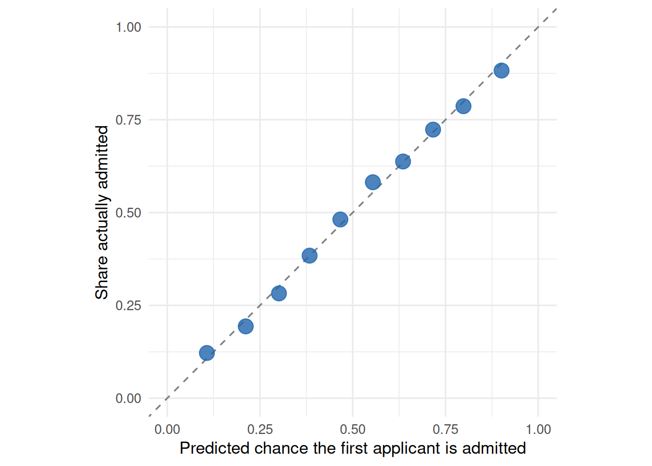
Start with one experiment, the immigration study the card opens on (the arithmetic below is for that one whichever you took). Fitting the model above to hainmueller_2014_immigrant – on four fifths of the 1,396 respondents at a time, predicting the fifth left out – gives a held-out probability for each of its 6,980 tasks: the chance that this respondent, whose choices the model never saw, picked the first of the two applicants. The model is often fairly sure. Its predictions run from 11% to 90% at the fifth and ninety-fifth percentiles, and across that range they are about right.
Code
cal <- example_pred |>mutate(bin =ntile(p_attr, 10)) |>group_by(bin) |>summarise(pred =mean(p_attr), obs =mean(y), n =n())ggplot(cal, aes(pred, obs)) +geom_abline(linetype ="dashed", colour = irw_grey) +geom_point(aes(size = n), colour = irw_blue, alpha =0.8) +scale_size_area(max_size =5, guide ="none") +coord_fixed(xlim =c(0, 1), ylim =c(0, 1)) +labs(x ="Predicted chance the first applicant is admitted",y ="Share actually admitted")
Figure 1: Held-out predictions for hainmueller_2014_immigrant, grouped into ten equal bins: the model’s average predicted probability that the first applicant was admitted against the share of those tasks in which the respondent did admit them. Points on the diagonal are predictions that come true at the rate claimed. Point size is the number of tasks in the bin.
To turn that into one number we compare two predictions of the same held-out choices: the attribute model, and a coin weighted to the share of first-applicant choices in the training respondents. The IMV converts each model’s average log-likelihood into the accuracy of a weighted coin that would earn it, and reports the relative gain.
The applicants’ attributes are randomized, so the coin is right 50% of the time – which is what makes a conjoint a clean test. The attribute model predicts these choices like a coin that comes up right 75.1% of the time, and the IMV is the gain over the baseline on that scale: 0.50. Nine attributes, none of which moves the average chance of admission by more than 0.28, together carry half again as much predictive accuracy as knowing nothing at all.
That is a lot, and this experiment is not typical: 91% of the conjoint experiments in IRW come out below it.
How much do the attributes explain?
Across 728 experiments the median IMV of the attribute model over a coin flip is 0.30. In accuracy terms, the median attribute model predicts a held-out choice like a coin that comes up right 67% of the time, against 51% for the baseline. That is a substantial amount for a randomly assembled bundle of five or ten features: knowing nothing about a respondent, and only what the two profiles look like, gets you most of the way from a coin flip to two choices in three.
The spread is wide. Eight in ten experiments fall between 0.13 and 0.5, and designs with more attributes are not more predictable (Spearman \(\rho\) = -0.02 between the IMV and the number of attributes). More attributes give the model more to work with but also more ways for a respondent to trade one against another, and the two appear to cancel.
Code
# The four experiments a reader can take, labelled in the words the menu uses.q1_widget <- q1 |>filter(table %in% widget_tables) |>left_join(tibble(table =c("hainmueller_2014_immigrant", "tellez_2021_peace_packages","laterzotingley_2024_crime_national", "chen_2025_bere_barley_scot"),tag =c("immigrants", "peace agreements", "candidates", "barley flour")),by ="table")p1 <-ggplot(q1, aes(n_attr, imv_attr,text =paste0(table, "<br>IMV = ", round(imv_attr, 3),"<br>attributes: ", n_attr, "<br>usable tasks: ", n_tasks_used))) +geom_jitter(width =0.15, height =0, colour = irw_blue, alpha =0.7, size =2) +geom_hline(yintercept = q1_med, linetype ="dashed", colour = irw_grey) +geom_point(data = q1_widget, colour = irw_red, size =3.5) +scale_x_continuous(expand =expansion(mult =c(0.03, 0.12))) +labs(x ="Number of attributes", y ="IMV, attributes over a coin flip")# ggplotly centres geom_text, so the four tags are plotly annotations instead,# anchored to the right of their point.ggplotly(p1, tooltip ="text") |>layout(annotations =lapply(seq_len(nrow(q1_widget)), function(i) list(x = q1_widget$n_attr[i], y = q1_widget$imv_attr[i], text = q1_widget$tag[i],xref ="x", yref ="y", xanchor ="left", yanchor ="middle", xshift =8,showarrow =FALSE, font =list(color = irw_red, size =11),bgcolor ="rgba(255,255,255,0.78)", borderpad =1)))
Figure 2: Held-out IMV of the attribute model over a coin flip, one point per experiment, by the number of attributes in the design. The dashed line marks the median. The red points are the four experiments the card above offers, which were picked to span this range. Hover for the table.
Against the item side of the warehouse
An IMV of 0.30 is easier to read next to the same quantity computed the same way on ordinary item response data. There, across 193 dichotomous tables, knowing which item a person is answering raises held-out prediction by a median IMV of 0.085, roughly a quarter of what a profile’s attributes do for a choice.
Figure 3: Held-out IMV over a weighted coin: profile attributes in conjoint experiments, item difficulties in dichotomous IRW tables. One point per table; the diamond marks the median.
Two things keep that gap from being a like-for-like contest between designs. The first is the baseline. A forced choice between two randomly built profiles is a coin flip by construction, so the baseline accuracy is almost exactly 51%, and any predictive signal has room to show. Items are not balanced that way: the median dichotomous table here is already right 67% of the time by always guessing the more common response, and relative gains over a baseline that good are necessarily smaller (the item model reaches 77%). The second is what the features are. A conjoint’s attributes are the whole stimulus, varied on purpose across the range the designer chose; an item’s difficulty is one number summarising a question somebody wrote for other reasons. A conjoint is, in effect, an experiment built to make the stimulus matter, and the comparison shows how much that design choice buys.
Which experiments are the attributes good for?
Table 1
What is being chosen
Experiments
Median IMV
Median held-out accuracy
Places
52
0.37
70% (from 52%)
Products and services
93
0.33
71% (from 51%)
Scenarios
38
0.31
68% (from 52%)
Organisations
25
0.31
67% (from 51%)
People
272
0.30
66% (from 51%)
Policies
234
0.27
66% (from 51%)
Messages
14
0.26
63% (from 51%)
The conjoint literature is dominated by choices between people – candidates, immigrants, job applicants – and between policies, but those are not where the attributes do the most work. Choices between things, places to live and products to buy, are the most predictable, and choices between policies and between political messages the least. A plausible reading is that a profile’s attributes come closer to exhausting what there is to know about a product than about a policy or a candidate, where what a respondent brings to the choice matters more.
Even so, the differences between kinds of choice are small next to the variation within them, and that is the more striking fact. At the top, chen_2025_bere_barley_scot reaches an IMV of 0.82, predicting held-out choices 91% of the time from 6 attributes; at the bottom, 10 experiments with designs of much the same size do not beat a weighted coin at all. What the attributes explain is a property of the particular experiment, not of the method.
Limitations
One model of the attributes. The model is additive in the attribute dummies with a single ridge penalty, so interactions between attributes, and the restrictions some designs place on which combinations can appear, are only approximated. A model that used them would predict somewhat better, so these numbers are a floor on what the attributes can do.
AMCEs average over indirect comparisons. The AMCE of one level against another pools the tasks where the two met with tasks where each met some third level, which makes it a transitive summary of the levels even when head-to-head choices are not. Abramson et al. (2022) propose an estimand restricted to direct comparisons, the average feature choice probability, and their first application is country of origin in the immigration experiment used here: the AMCE for France against Poland is indistinguishable from zero, while in direct comparisons respondents favour Poland by about 0.11. So the widget’s reference points describe averages, not which profile wins a given pairing. Bansak et al. (2023) defend the AMCE for the election-outcome quantities it was built for. The same point reaches the predictive question: our model scores each profile from its own attributes alone, so it cannot represent a choice that turns on the pairing, and whatever structure of that kind exists here is counted as noise rather than signal. We do not switch estimands because direct comparisons are a small share of a uniformly randomized design, and most tables here are not large enough to support them.
Comparing two designs, not two estimates. The conjoint and item-response numbers are the same calculation, but their baselines are not equally easy to beat (a forced choice starts at 51%, the median dichotomous item table at 67%), and item difficulty is a thinner description of an item than a profile’s attributes are of a profile. Read the gap as a difference between kinds of design, not as a measurement of one quantity in two places.
A random, unmatched item sample. The 193 item-response tables are a random draw from dichotomous core tables, not matched to the conjoint experiments by sample, domain or length.
Forced choices only. Ratings, opt-out tasks and designs with one or three profiles are left out, as are tables with fewer than 500 usable tasks. The screen keeps 728 of the 1143 conjoint tables in IRW.
Zero and negative values are kept. 5 conjoint tables come out slightly below zero, where the attribute model predicts held-out respondents worse than the training base rate does, and 5 come out at exactly zero, where neither model beats a fair coin and the IMV’s accuracy scale floors both at 50%. They are left in, since dropping them would bias the median upward.
One version of the source. Everything here is irw_conjoint v4.2 and irw_conjoint_2 v1.4. Later versions will add experiments; rerunning means changing the version strings at the top of conjoint_compute.R.
One table left out.joo_2026_descriptive_rep meets the criteria but is excluded: in its deposit every respondent’s chosen candidate has the same position in all six tasks, so its outcomes do not line up with its profiles.
The widget. Each experiment ships a random 250 of its tasks, and the estimator is a simple difference in choice rates rather than a model. Its reference points are the published AMCEs for the immigration experiment and the same simple difference over all respondents for the other three, whose standard errors, unlike the published ones, ignore the clustering of tasks within a respondent. The four experiments were chosen to be readable and to spread across the range of results, so they are not a random sample of IRW.
These results were computed against approximately IRW v584 (the corpus as of October 17, 2026).
NoteHow this version was determined
The version was inferred from when the results were computed, not recorded during the run, so it may be off by a version or more. To pin data to an exact version, use irw_use_version().
Results were computed on October 17, 2026 from irw_conjoint v4.2, irw_conjoint_2 v1.4 and irw_meta v44.0. To regenerate:
# 1. Re-run the compute script (from the project root)source("vignettes/conjoint_compute.R")# 2. Re-render this pagequarto::quarto_render("vignettes/conjoint.qmd")
Abramson, Scott F., Korhan Kocak, Asya Magazinnik, and Anton Strezhnev. 2022. “Detecting Preference Cycles in Forced-Choice Conjoint Experiments.” Unpublished manuscript. September.
Bansak, Kirk, Jens Hainmueller, Daniel J. Hopkins, and Teppei Yamamoto. 2023. “Using Conjoint Experiments to Analyze Election Outcomes: The Essential Role of the Average Marginal Component Effect.”Political Analysis 31 (4): 500–518. https://doi.org/10.1017/pan.2022.16.
CHEN, Jianyu, Tareq Mzek, and Simone Piras. 2025. Dataset of Choice Experiment Surveys Assessing Consumers’ and Farmers’ Preferences for Five Underutilised Crops in Different European Countries. Zenodo. https://doi.org/10.5281/ZENODO.15420092.
Domingue, Benjamin W., Klint Kanopka, Radhika Kapoor, et al. 2024. “The InterModel Vigorish as a Lens for Understanding (and Quantifying) the Value of Item Response Models for Dichotomously Coded Items.”Psychometrika 89 (3): 1034–54. https://doi.org/10.1007/s11336-024-09977-2.
Domingue, Benjamin W., Charles Rahal, Jessica Faul, et al. 2025. “The InterModel Vigorish (IMV) as a Flexible and Portable Approach for Quantifying Predictive Accuracy with Binary Outcomes.”PLOS ONE 20 (3): e0316491.
Hainmueller, Jens, Daniel J. Hopkins, and Teppei Yamamoto. 2014. “Causal Inference in Conjoint Analysis: Understanding Multidimensional Choices via Stated Preference Experiments.”Political Analysis 22 (1): 1–30. https://doi.org/10.1093/pan/mpt024.
Laterzo-Tingley, Isabel, and Leah Christiani. 2024. “The ‘Tough-on-Crime’ Left: Race, Gender, and Elections of Law-and-Order Democrats.”Research &Amp; Politics 11 (3). https://doi.org/10.1177/20531680241261765.
Tellez, Juan Fernando. 2021. “Peace Without Impunity: Worldview in the Settlement of Civil Wars.”The Journal of Politics 83 (4): 1322–36. https://doi.org/10.1086/711555.