Bits per Item: How Much Does a Test Tell You About a Person?

A test is a sequence of questions asked about something we cannot see: not the person, who is right in front of us, but the trait we want to measure. Each answer narrows down where that person sits on it. Information theory counts that narrowing in bits, Shannon’s unit for the length of the shortest message that would tell someone the answer. One bit is what you learn from a yes/no question that splits the remaining possibilities in half, so a test worth two bits has done the work of two ideally placed yes/no questions about where the person stands, and a test worth ten has done the work of ten. We play this out on three real tests, then measure the bits delivered by more than two hundred dichotomous tests in the Item Response Warehouse, and close with three tests whose answers come in ordered categories.

Published

October 23, 2026

Note

This vignette — including the dataset search, the compute script, the analysis design, and the writing below — was produced largely by Claude (Anthropic), working from a task specification and with human review. Treat the methodological choices and interpretations accordingly, and check the compute script (bits_per_item_compute.R) directly if you’re relying on the numbers here.

Cutting up the population

Start with an imaginary test whose questions are perfect. People are spread along θ, the trait being measured, in the familiar bell shape. Each question is a cut: everyone above it answers right, everyone below answers wrong. Asking it tells you which side of the cut a person is on, and nothing else.

Click on the chart to place a cut (or use the slider), and watch the bits. The cuts chop the population into groups, and a person’s answers tell you exactly which group they are in. How much is that worth? Information theory measures it with entropy, written H: how uncertain you are about something before you find out, counted as roughly the number of yes/no questions you would need, on average, to pin it down. Here the something is which group a person is in. It has to be a which question: a trait like θ is continuous and can never be pinned down exactly, so we always count bits about which of a fixed set of groups a person falls in. Once the groups are fine enough, the number of bits a test delivers no longer depends on how fine they are, which is what lets us talk about a test’s bits at all. With perfect cuts the bits the test gives are exactly the entropy of the groups. Groups holding shares p of the population have H = −Σ p log2 p. One cut at the median makes two halves: 1 bit (each half holds p = ½ of people, so −½ log2 ½ − ½ log2 ½ = ½ + ½ = 1). Three cuts at the quartiles make four quarters: 2 bits (4 × −¼ log2 ¼ = 4 × ½ = 2). In general k cuts are worth at most log2(k + 1) bits, reached only when they make equal groups.

Then turn up the blur. A blurred cut is a real question: near the cut, people sometimes land on the wrong side, so the answer is partly luck. The luck is noise, and it comes off the top.

Some things to try:

  • Median, then add another cut at 0. The second cut adds nothing: it asks a question that has already been answered. Redundancy is the first way bits are lost.
  • Quartiles. Each cut’s “bits added” depends on what was there before. The first cut is worth a full bit; the next two split halves, and are worth half a bit each, because each only matters for the half of the population it falls in.
  • 3 near the median. Cuts at −0.1, 0 and +0.1. The outer two each split off a sliver of about 4% of people, so together the three are worth 1.40 bits, well short of the 2 that three spread-out cuts can give. A cut close to an existing one asks nearly the same question.
  • 3 in the low tail. Each cut splits off a sliver. Cuts where few people are say little about most people.
  • Quartiles, then blur. The bits fall below 2 even though the cuts are perfectly placed. Near each cut the answer is now partly luck, and luck says nothing about the person. The next section measures that luck.
  • Numeracy test. Cuts at the difficulty of each of its items, blurred by its typical slope. They pile up between about −1 and −0.5, and blurred, the whole test is worth little more than one well-placed perfect question. The real test, with each item’s own slope, carries 1.18 bits.

Answer patterns

Everything on this page comes from one object: the answer pattern, which we denote X. It is the string of right and wrong answers a person gives, X = (X1, …, XJ) for a test of J items, with Xj = 1 for a right answer to item j and 0 for a wrong one. List every pattern a test could produce and two quantities decide how much the test tells you about a person:

  • Spread, H(X): how varied the patterns are across the population.
  • Noise, H(X | θ): how varied they would be for one value of θ, as if a person at that θ answered again and again.

The information about the person is what is left: I(θ; X) = H(X) − H(X | θ), in bits.

Both are entropies, computed from pattern probabilities. Write p(x) for the share of the population that would give pattern x, and p(x | θ) for the chance that a person at θ gives it. Then

  • H(X) = −Σx p(x) log2 p(x), summed over all 2J patterns. Under an IRT model, p(x) is the average of p(x | θ) over the population: p(x) = ∫ p(x | θ) g(θ) dθ, with g the distribution of θ.
  • H(X | θ) = ∫ g(θ) [−Σx p(x | θ) log2 p(x | θ)] dθ: the same entropy for a person at a fixed θ, averaged over the population. Because the model treats answers as independent once θ is fixed, p(x | θ) is a product over items and this reduces to a sum over items, ∫ g(θ) Σj h(Pj(θ)) dθ, where Pj(θ) is the chance of a right answer to item j and h(p) = −p log2 p − (1 − p) log2(1 − p).

These entropies have a concrete reading as message lengths (Chris Olah’s Visual Information Theory builds this up with pictures). The shortest code for sending a message that we observed pattern x is −log2 p(x) bits long, so H(X) is the average length of that message when the receiver does not know θ, and H(X | θ) is its average length when both sides know θ. The difference is how much knowing θ shortens the message, which is the same as how much the message tells you about θ. Equivalently, if you had to send which of the 64 slices someone is in, seeing their answers first would cut that message by I(θ; X) bits on average.

Our p(x) is the model’s version of what the Dutch identity vignette calls manifest probabilities. There they are estimated from how often each pattern was actually observed, and then modelled; here they are computed from the fitted IRT model. The dots in the five-question chart below are the observed version. That vignette studies their shape; this one counts their spread. The worked example under the five-question chart below goes through every step of this calculation for one pattern.

The cuts above were the special case with no noise. Now we build this up on a real numeracy test: one question first, then three, five, and the whole test.

One question

With one question there are only two patterns, right and wrong. To picture the population we cut θ, the trait being measured, into 64 slices, each holding the same share of people: narrow in the crowded middle, wide in the thin tails. Pinning down one slice out of 64 would take 6 bits, since 26 = 64.

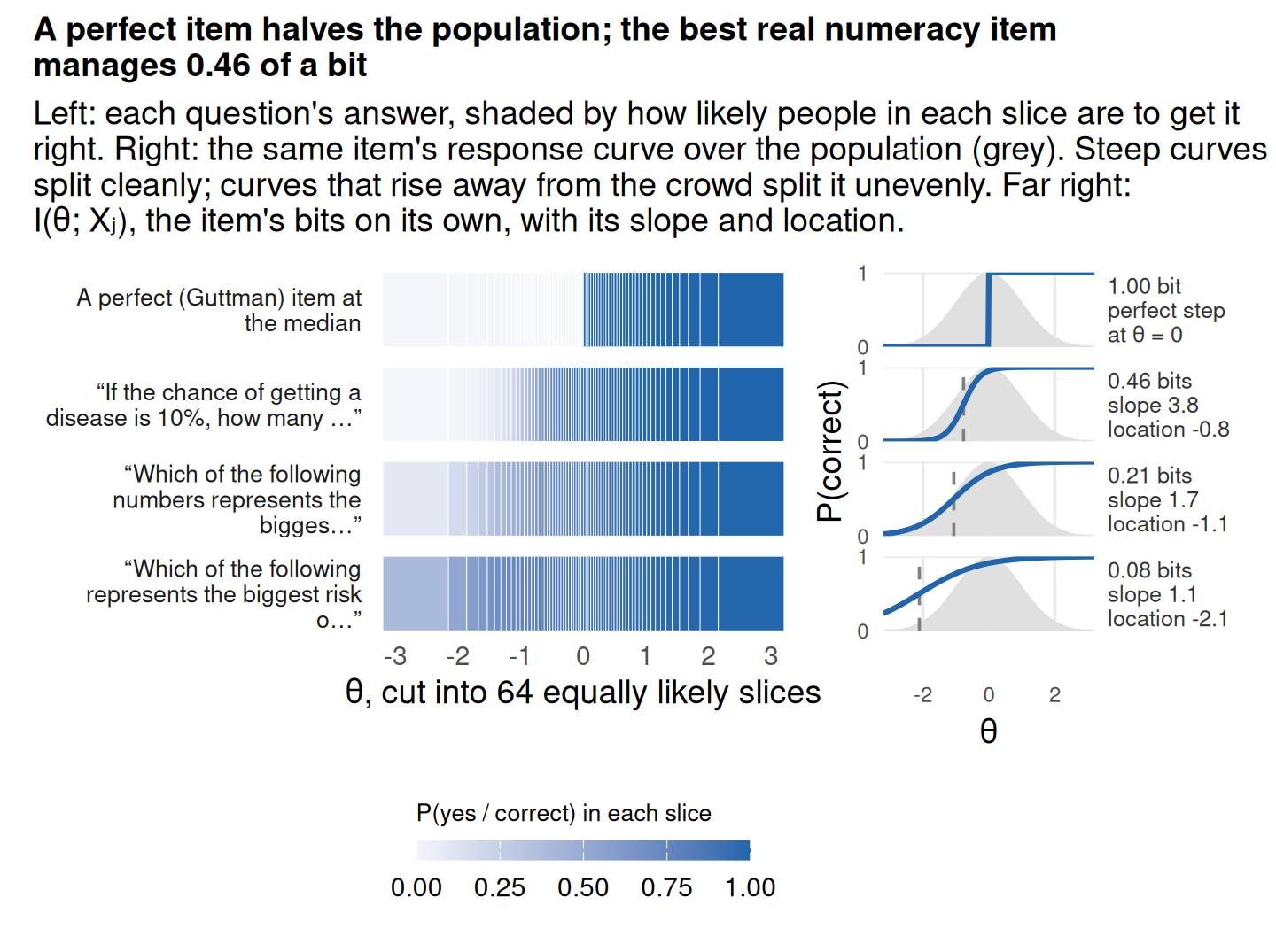
A bit is the information in the answer to a question whose two answers are equally likely and which splits the possibilities cleanly. The top row of the figure does exactly that: it cuts 64 slices to 32. Real items don’t split the sample so cleanly, for two reasons. Their split is blurred, because people in the same group sometimes answer differently. And their split is often off-centre, because easy items mostly separate the lowest groups from everyone else. Both can be read off the item response curves on the right: a shallow slope blurs the split, and a curve that rises away from the bulk of the population (grey) splits it unevenly. In pattern terms, the spread is the entropy of the answer across the population, the noise is the entropy of the answer for someone at a fixed θ, and the information is the gap: I(θ; Xj) = h(P̄j) − Eθ[h(Pj(θ))], with h(p) = −p log2 p − (1−p) log2(1−p). Neither term can exceed one bit.

Three questions

Top: hover anywhere on θ, or read straight up from it, to see the mix of patterns a person there would give, answering again and again. Bottom: the same mix averaged over the population. Bits = spread of the bottom bars, H(X) = 2.24, minus the average spread of a vertical slice of the top panel, H(X | θ) = 1.48. Items, in pattern order: numeracy8a, numeracy8b, numeracy9.

Read the top panel straight up from any point on θ. Far to the left almost everyone gives 000; far to the right almost everyone gives 111. In between, a person at a fixed θ could give several patterns, and which one comes out is partly luck. Perfect cuts would allow only four of the eight patterns: the ones in which every item a person gets right is easier than every item they get wrong. Blur is what lets the other four appear. That luck, which has nothing to do with differences between people, is the noise, H(X | θ) = 1.48 bits on average. The bottom panel is what you see when you do not know θ: the mix averaged over everyone, whose entropy, the spread, is H(X) = 2.24 bits. The information is the gap, 0.76 bits, and it comes entirely from the mix changing along θ. If every θ produced the same mix, the top panel would be flat bands, the spread and the noise would be equal, and seeing a pattern would tell you nothing about the person.

In the language of measurement error, 0.76 bits is how far three answers narrow down θ. If θ and the evidence about it were jointly normal, each bit would halve the standard error, so 0.76 bits would leave an error of 2−0.76 ≈ 0.59 population SDs, a reliability of about 0.65. Computed exactly from the model, the typical error after these three answers (the root-mean-square posterior SD) is 0.62 SDs. The two differ a little because answers are not normal; Reliability in bits takes this up.

Five questions

Bars: the model’s probability of each pattern. Dots: the share of the 2,778 respondents who actually gave it. Items, in pattern order: numeracy8a, numeracy8b, numeracy9, numeracy1, numeracy3. Hover over a bar to see its pieces: which answers the pattern contains, who tends to give it, and how much it contributes to the spread, to the noise, and to the net bits. Summed over the 32 bars, the spread is 3.70 bits and the noise 2.75, leaving 0.95 bits about the person. Most of the spread is noise; a person’s response pattern offers only limited information about θ.

The five items’ bits taken one at a time add up to 1.55, more than the 0.95 they give together: they partly ask the same thing. The overlap, 0.60 bits, is exactly Σj H(Xj) − H(X), which measures how far the patterns are from what independent items would produce. That is the departure from the independence model in the Dutch identity vignette, counted in bits. The trait that makes items agree with each other is also what makes their information overlap.

1. The chance of the pattern for one person. The model gives each item a probability of a correct answer that depends on θ. For a person at a given θ, the chance of the whole pattern is the product of the chances of its five answers, because the model treats answers as independent once θ is fixed. Here it is for three people:

item answer θ = −1 θ = 0 θ = +1
numeracy8a correct 0.292 0.951 0.999
numeracy8b correct 0.285 0.810 0.979
numeracy9 correct 0.298 0.771 0.964
numeracy1 correct 0.179 0.468 0.780
numeracy3 incorrect 0.983 0.902 0.589
product 0.004 0.250 0.433

2. Average over the population. Do the same at every θ and average the products, weighting each θ by how many people sit there (a normal curve, on an 81-point grid). That average, 0.214, is the height of the bar. 20% of respondents actually gave this pattern.

3. Spread. Each bar adds −p log₂ p to the spread: here −0.214 × log₂ 0.214 = 0.476 bits. Summed over all 32 bars that is H(X) = 3.70 bits.

4. Noise. The same calculation within each θ, using the products from step 1 instead of the average, then averaged over the population: 0.354 bits from this pattern, H(X | θ) = 2.75 bits in all. This is how unpredictable the pattern is even for someone whose θ we know.

5. Information. Spread minus noise: I(θ; X) = 3.70 − 2.75 = 0.95 bits. A single bar’s net can be negative; only the total has to be positive.

The whole test

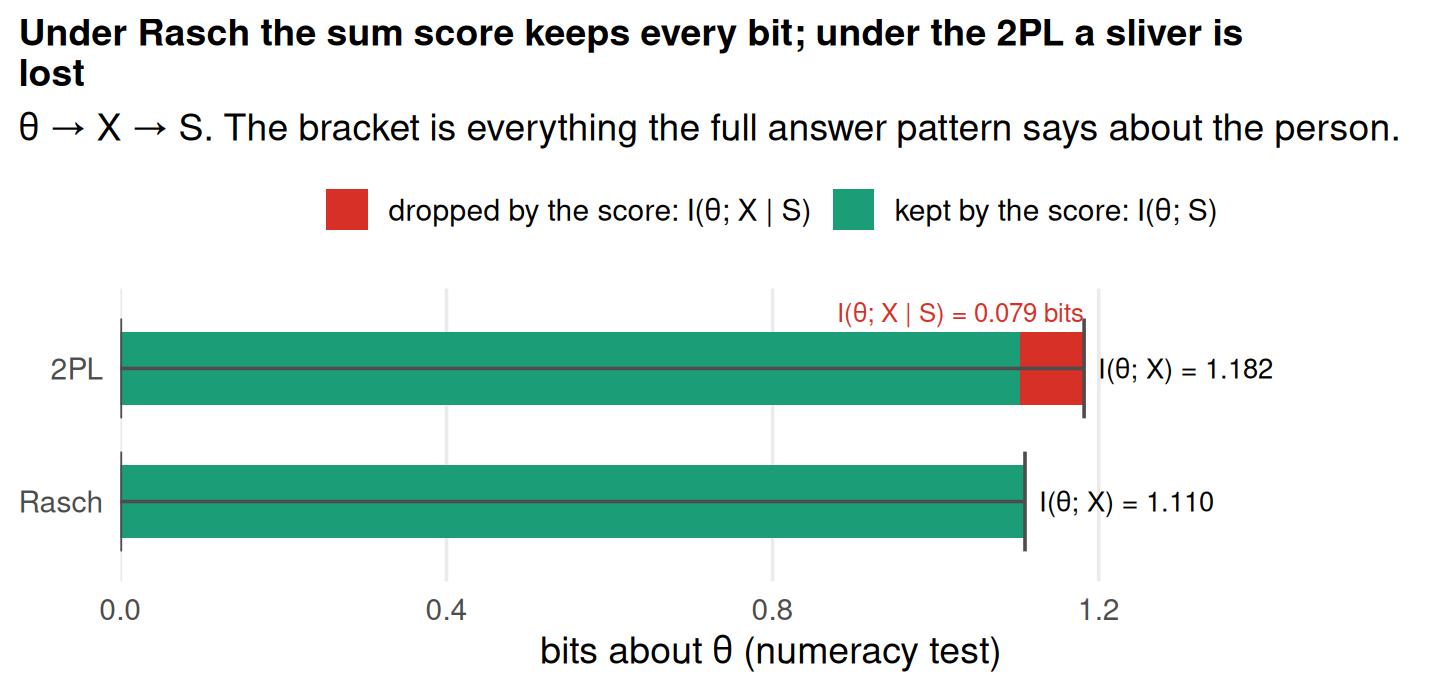
The numeracy test has 11 items, so 2,048 possible patterns: too many to draw, but not too many to count. The same calculation gives a spread of 8.13 bits, noise of 6.94 bits, and so 1.18 bits about the person. Adding six items to the five above bought about 0.23 bits more. The sum score gathers the 2,048 patterns into 12 piles, one per score (the score distribution plotted in the Dutch identity vignette, whose Section 4 shows its shape under the Rasch model), and keeps 1.10 of those bits; Is the sum score enough? asks what the piling loses. For long tests the patterns cannot be listed, and the same quantities are estimated by simulation (see How the warehouse numbers were computed).

One person, one answer at a time

So far everything has been an average over the population. Now follow one person through the test: what each answer buys, how surprising each answer is, and how fast the uncertainty about them falls.

Guess the person

Somewhere in the population below is one person, and your job in this game is to find out which of the 64 slices they are in by asking questions from a real test. Before any question there are 6 bits to find. After each answer the slices are re-shaded, darker where the person is now more likely to be, and a line traces the same thing as a density over θ. The counter shows how many bits that answer bought.

Pick a question from the table; they are ranked by how many bits they are expected to give. Then either answer it yourself, as the person might, or let the simulated person answer. At the start we secretly draw one simulated person from the population; they answer with the probabilities the model gives someone in their slice. You can reveal where they are at any point. The “best” and “worst” buttons ask the remaining question with the most or the fewest expected bits, and the simulated person answers it.

A few things show up quickly. No real question is worth anywhere near a full bit: the best ones promise about half a bit at most. A full bit would take a perfectly sharp (Guttman) item whose cut falls exactly in the middle of what we currently believe, splitting the remaining possibilities in half. Questions lose value as you go, because the easy distinctions have already been made. And now and then the shading spreads out after an answer. That happens when the person says something the model did not expect.

Surprise

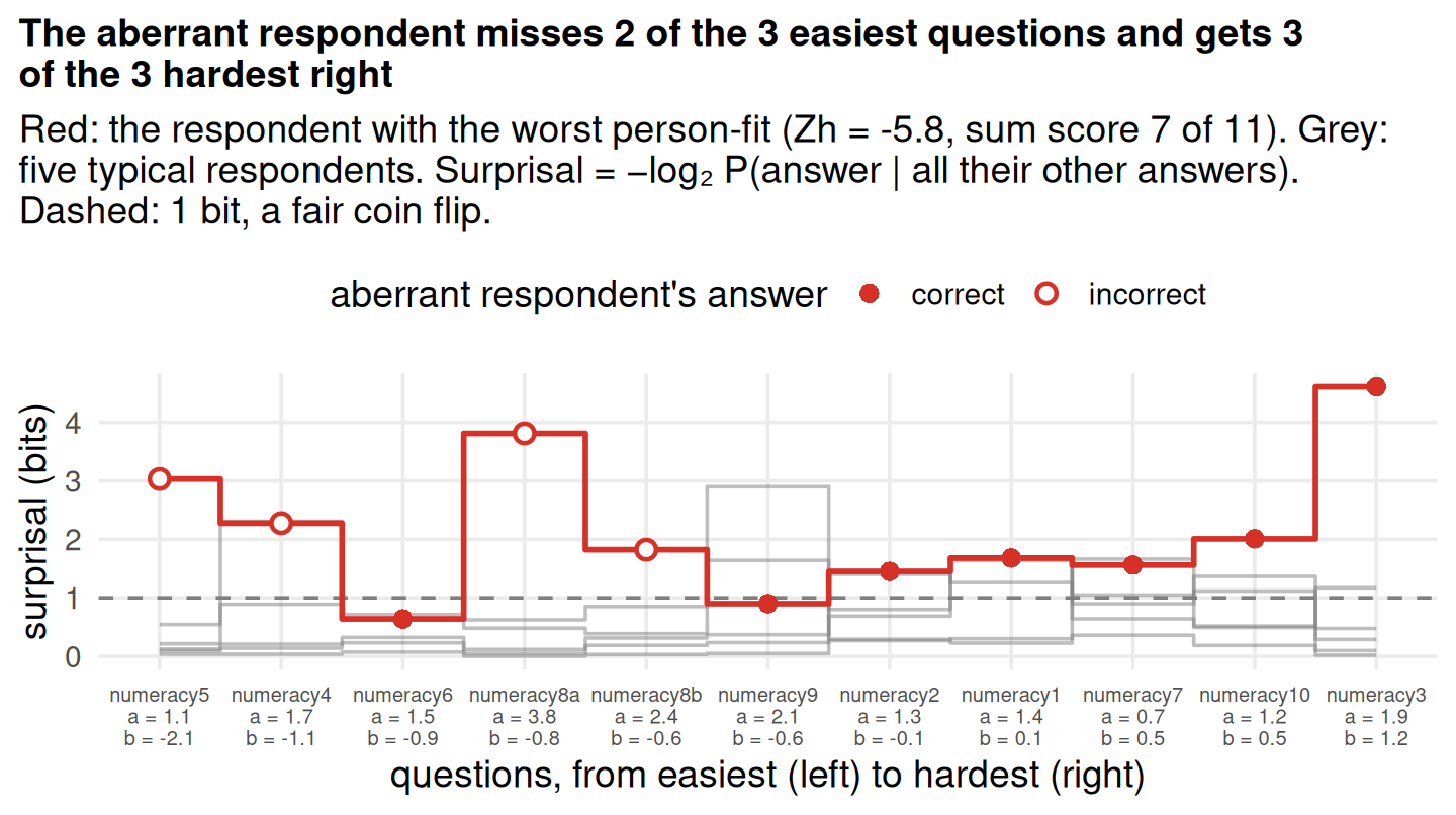
The surprisal of an answer is −log2 of the probability the model gave it. An answer the model thought had a 50% chance costs 1 bit of surprise; one it thought had a 1-in-8 chance costs 3 bits. Here each answer is judged against everything else the person answered: hide one answer, work out from the others where the person probably sits, and ask how likely the hidden answer was from there. Nothing depends on the order of asking; the questions are lined up from easiest to hardest only so the pattern is easy to read.

Most answers from typical respondents sit around or below a bit, because their other answers place them well and each answer agrees with that placement. The red respondent’s answers disagree with each other. The rest of the pattern says “able enough for the hard questions”, which makes the misses on the easy ones very unlikely, and vice versa, so the surprise lands on exactly the answers that do not fit. This is the logic of person-fit statistics such as Zh, one answer at a time.

Surprisal depends on an item’s slope as well as its difficulty. The easiest question, numeracy5 (a = 1.1, b = -2.1), is also one of the flattest, so even fairly able people miss it now and then; the red respondent’s miss costs 3.0 bits. Their miss on numeracy8a (a = 3.8, b = -0.8), which is harder but much steeper, costs 3.8: anyone the rest of the answers place above its location almost never gets it wrong. Leaving one answer out also changes the evidence. A miss on a steep item pulls the estimate of θ down more than a miss on a flat one, so it makes the person’s other misses look less surprising.

Elsewhere on the page, as in the game above, surprisal is judged against the answers so far. That version depends on order, and it adds up: the surprisals of one ordering sum to the surprisal of the whole pattern. The leave-one-out version does not add up that way, but it gives each answer one number whatever the order, which is what a question about fit needs.

Watching uncertainty fall

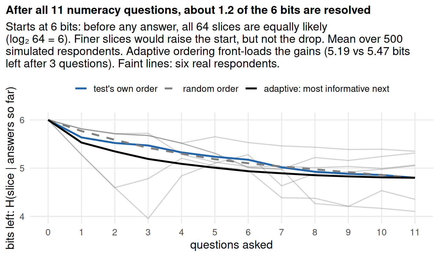
The faint lines for real respondents do not only fall. A single answer can increase the uncertainty, and it mostly happens after a surprising answer: one that the person’s answers so far made unlikely. Such an answer pulls belief away from where it had settled and spreads it back out. The red respondent from the Surprise section has the largest of these rises. On average, though, an answer can never add uncertainty, which is why the mean lines only fall.

Every order ends in the same place, because the same answers have been given. What changes is how fast you get there. Asking the most informative question next, given what is already known, buys in three questions what the fixed order needs several more to reach. This is the logic of computerised adaptive testing, and of Wordle solvers. The ending point is the real news, though: a full pass through this test leaves most of the uncertainty about which of 64 groups a person belongs to unresolved.

What one answer does to the belief

The guessing game above kept score with entropy: how many bits of uncertainty about θ are left, and how many an answer removed. That score measures how much an answer narrowed the belief about θ, the drop in the entropy of the posterior over the slices. It says nothing about where the belief went. There is a second way to score an answer, by how far it moved the belief rather than by how much it narrowed it. The distance from the belief before an answer, Q, to the belief after it, P, is the Kullback–Leibler divergence

\[D(P \,\|\, Q) = \sum_{\text{slices}} P(\text{slice}) \log_2 \frac{P(\text{slice})}{Q(\text{slice})},\]

the expected number of extra bits it costs to encode draws from P with a code built for Q. It is never negative, and it is zero only when nothing moved.

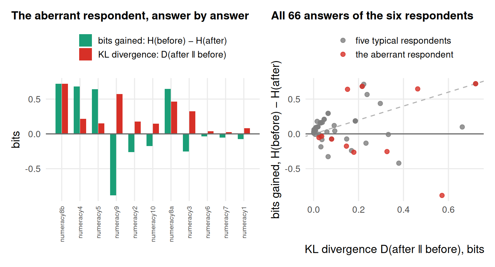
The figure scores every answer of six real respondents both ways, once by entropy removed and once by divergence. The two scores agree on average and disagree answer by answer. Averaged over the answers a person might give, both equal the item’s expected bits, I(slice; Xj | answers so far), so the mean curves in Watching uncertainty fall would look the same under either. But a single answer is different. The left panel replays the aberrant respondent from the Surprise section in the test’s own order. Their answer to numeracy9, a correct answer that the belief at that point gave only a 17% chance, moves the belief by 0.57 bits of divergence while adding 0.88 bits of entropy: an answer that runs against the belief drags the posterior a long way and, in doing so, spreads it back out. On the first answer the two bars are equal, and always will be: from a flat belief over N slices, D(after ‖ flat) = log2 N − H(after), which is exactly the entropy removed. After that they come apart. The right panel makes the pattern general. The divergence is never negative, so no point lies left of zero; the bits gained can be, and the points below the horizontal line are the answers that left the person less pinned down than before, typical and aberrant respondents alike. The two scores are on the same scale (both average to the item’s expected bits) but they measure different things: the dashed line of equality is a reference, not a bound.

Most of the page’s quantities are divergences in disguise. Mutual information I(θ; X) is D(P(θ, X) ‖ P(θ)P(X)), the divergence from the joint distribution to the one it would have if the test told you nothing. The redundancy of the five questions in Five questions, Σj I(θ; Xj) − I(θ; X), is the divergence from the fitted model to the model in which the items are independent. The surprisals of the Surprise section, summed over a person’s answers, are the divergence from their empirical answer distribution to the model’s. And the loss from merging an item’s categories, later on the page, is the expected divergence from the full conditional distribution to the merged one. One idea, several units of measurement.

NoteWhich information? The quantities on this page

Several different “bits” have now appeared, and the rest of the page leans on the differences between them. They are not interchangeable.

  • I(θ; X): what the full answer pattern says about the person, on average over the population. This is “the test’s information” in the warehouse figures.
  • I(θ; Xj): what one item says on its own. Items repeat each other, so these do not add up to the test’s total: I(θ; X) ≤ Σj I(θ; Xj).
  • I(θ; Xj | answers so far): what one more item is expected to add, given the particular answers already seen. These are the “expected bits” in the game above, and the same item is worth less once earlier answers have done its job.
  • Bits gained by one answer: H(θ | before) − H(θ | after). This is a realised change, not an average, so it can be negative. Averaged over possible answers it equals the expected bits.
  • Surprisal: −log2 P(answer | answers so far), how unexpected one answer was. The Surprise section conditions instead on all the person’s other answers.
  • I(θ; S) and I(θ; X | S): what the sum score keeps, and what it drops.
  • KL divergence D(P ‖ Q): Σ P log2(P/Q), the cost in bits of using a code built for Q when the truth is P. Never negative. Mutual information, the realised movement of the belief after an answer, the redundancy between items, and the loss from merging categories are all divergences; see What one answer does to the belief.

Now, the whole warehouse

So far one test has carried the story: an 11-item numeracy test (the game also offers two others). From here on we zoom out from one table to a much bigger pool, running the same calculations on 240 tests from the Item Response Warehouse, so that the questions become ones about tests in general: how many bits a typical test delivers, and what drives the differences. The first part below says which tables went in and how they were processed; the rest shows the results.

How the warehouse numbers were computed

Selection started from every dichotomous IRW table with 5–60 items and at least 500 respondents. Each candidate was then fetched and checked. Tables with waves or treatment arms were restricted to one administration: the earliest wave, then the control arm. Tables with repeated person–item rows (trial-level tasks) were excluded, as were tables with response density below 0.8. ENEM tables were left out for this version. That left 241 tables, of which 240 produced results (1 failed: ai_fear_dong_2026_incentive, where every respondent gives the same answer to every item). Tables with more than 10,000 respondents were randomly subsampled to 10,000 (36 tables). Items answered by fewer than half the respondents, and items with no variance, were dropped.

For each table we fit Rasch and 2PL models with mirt, using a lognormal(0, 1) prior on 2PL slopes, and read the latent distribution from each fit: N(0, σ²) with σ² estimated for Rasch, N(0, 1) for 2PL. All quantities are integrals over that distribution on an 81-point grid spanning ±6 SD. In bits:

  • I(θ; S), the information in the sum score, via the Lord–Wingersky recursion.
  • I(θ; X), the information in the full response pattern. It is exact by enumerating all patterns when there are 16 or fewer items, and Monte Carlo above that (standard error below 0.005 bits). For Rasch the two are equal, because the sum score is sufficient.
  • H(X | θ), the noise, and H(X) = I(θ; X) + H(X | θ).
  • Marginal reliability, the reliability of EAP sum scores, and their Gaussian bit equivalents −½ log2(1 − ρ).
  • Per-item bits, length curves, and a sum-score model check.

Validation checks (entropy edge cases, single items under 1 bit, Rasch sufficiency, I(θ; S) ≤ I(θ; X) on every table, Monte Carlo against enumeration, binned against continuous, simulation recovery, grid stability) are in bits_per_item_checks.R. All passed.

How many bits do tests carry?

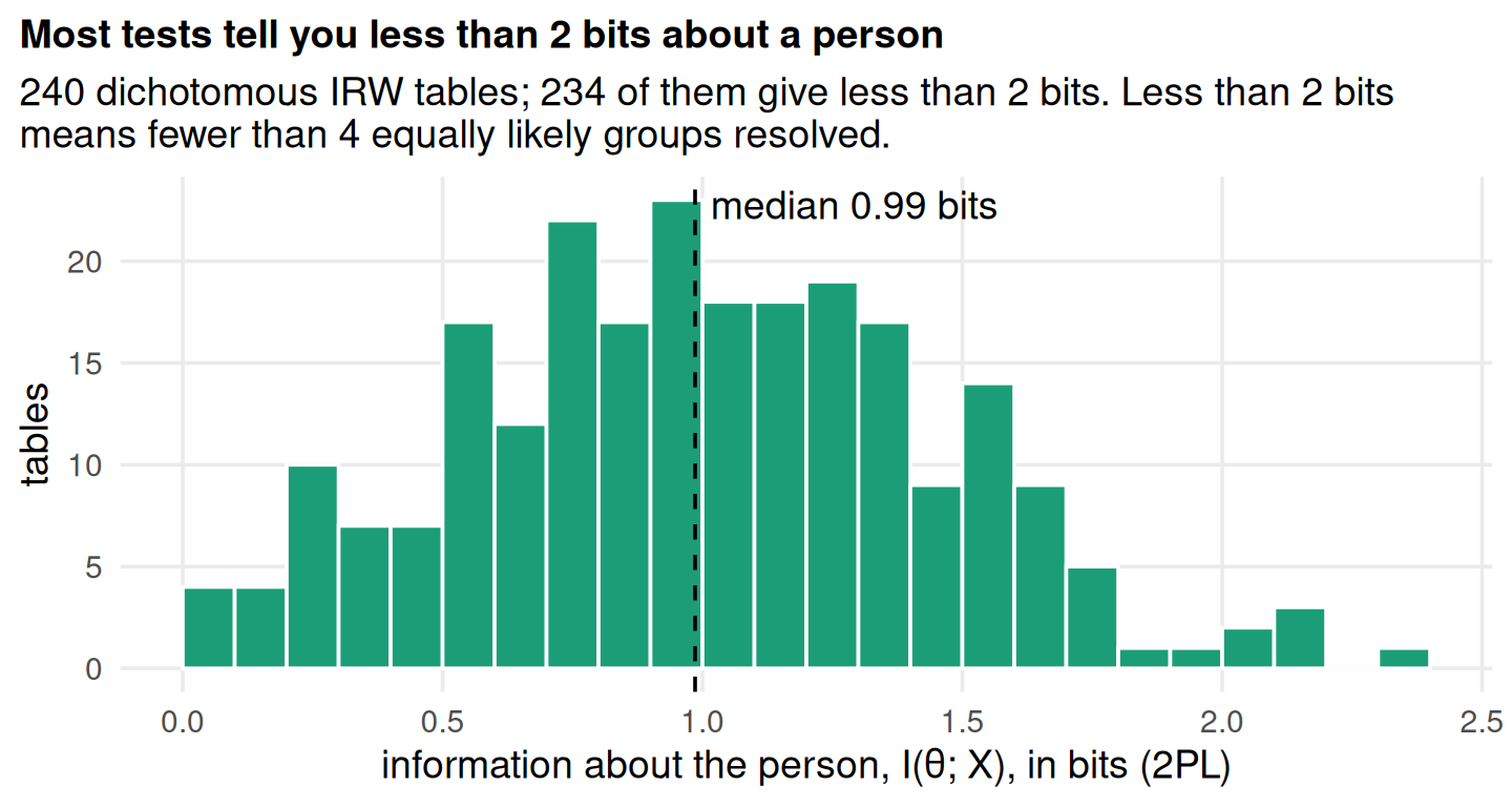
Across 240 tables, the median test delivers 0.99 bits about the person it measures: about as much as learning which half of the population someone is in. The most informative, gilbert_meta_72 (47 items), reaches 2.38 bits. Tests are short and noisy relative to the population spread, and bits grow only logarithmically with precision: each extra bit requires halving the standard error.

The dashed line is a hard ceiling. On a single trait, n items that never make mistakes can produce only n + 1 different answer patterns, so they carry at most log2(n + 1) bits, reached when the items cut the population into n + 1 equal parts. Real tables sit far below it, a median of 26% of the way up. The missing bits are lost to noise, not to test length: answers are probabilistic, so the same person could produce many patterns.

The solid line is a smoothed average (loess, with a band of ±2 standard errors). Typical bits do rise with length, from about 0.7 at 5 items to 1.1 at 20 and 1.4 at 40, but far more slowly than the ceiling, which climbs from 2.6 to 5.4 bits over the same range. Beyond about 40 items the line levels off, though only 17 tables are that long, so the band widens there. Diminishing returns follows the same question inside individual tests.

Reliability in bits

Reliability and bits measure related things. If θ and a score were jointly normal, with the score’s correlation with θ equal to √ρ, the information between them would be exactly −½ log2(1 − ρ). Item responses are binary, not normal, so the question is how far real tests depart from that curve, and why. We look first at synthetic tests, where we control the items, and then at the warehouse.

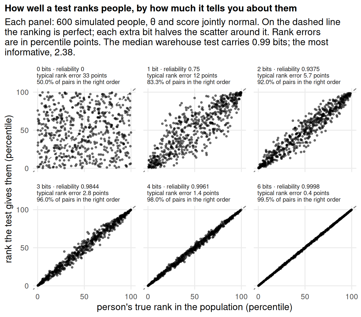
Turning that formula around, b bits corresponds to a reliability of 1 − 4−b. To see what that buys, simulate people from the Gaussian picture and compare each person’s true rank with the rank the score gives them.

Most of what a ranking needs arrives in the first bit or two: one bit already puts five pairs in six in the right order. The panels show the Gaussian picture, which is the dashed curve below. The warehouse tests sit a little above that curve, so their bits are only approximately where they land in these panels.

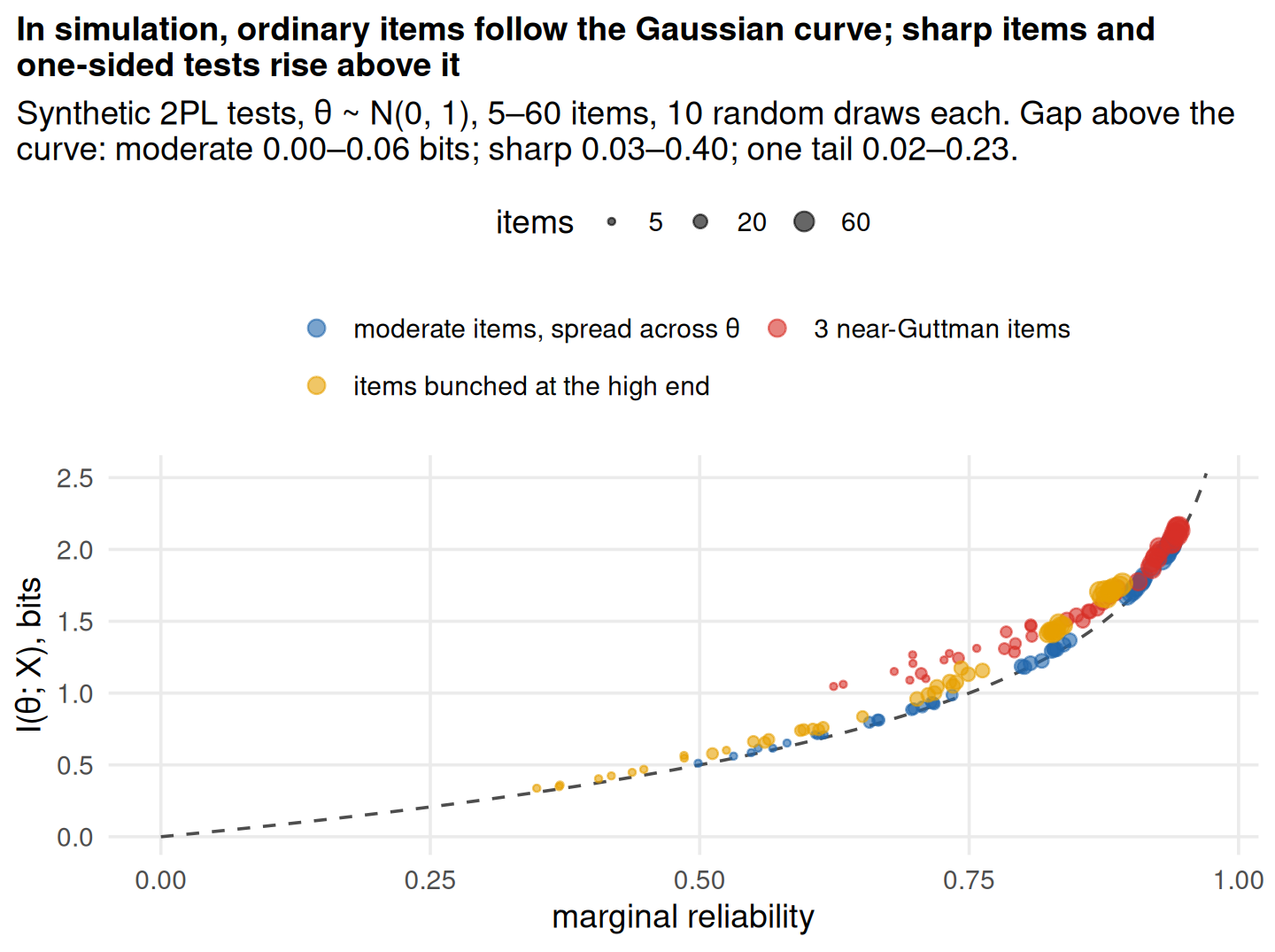
Reliability sees only the variance of what is still uncertain about θ after the answers. Bits see its whole shape. Among all distributions with a given variance, the normal is the most uncertain one, so the Gaussian formula −½ log2(1 − ρ) describes the worst case: with θ normal, the true information is at least that much, and equal to it only when every posterior is normal and has the same width. Real tests break that in two ways, the two departures in the simulation below.

Sharp items leave lumpy posteriors. Take one perfect cut at the median. It is worth exactly 1 bit: you learn which half the person is in. But the top half of a normal distribution has variance 1 − 2/π ≈ 0.36, so as a reliability the cut is worth only 0.64, and the Gaussian formula turns that into 0.73 bits. The hard edge at the cut is very informative, but it does not shrink the variance much.

Uneven precision. A test whose items bunch at one end is precise there and vague elsewhere. Reliability averages the error variances; information, in effect, averages their logarithms. The average of the logs is larger than the log of the average, so uneven precision is worth more bits than its average error suggests, and the gap grows as the unevenness does.

A technical note: the marginal reliability used here is built from Fisher information, a large-sample approximation, rather than from exact posterior variances. The two track each other closely in these data, but the guarantee above is strictly for the posterior-variance version.

With ordinary items, moderately discriminating and spread across θ, the Gaussian formula is close: reliability tells you the bits. Two departures push tests above the curve. A few near-Guttman items split the population almost deterministically. That is worth bits a reliability coefficient, built on squared error, undercounts. The effect is largest in short tests (0.31 bits at 5 items) and fades as ordinary items accumulate (0.06 at 60). Items bunched in one tail make the score precise at one end and vague elsewhere, and that gap grows with test length (0.04 → 0.18 bits).

Dashed line: −½ log₂(1 − ρ), the information if θ and its estimate were jointly normal. Hover a point for the table.

On the Gaussian curve, a reliability of .80 is worth 1.16 bits, .90 is worth 1.66, and .95 is worth 2.16. The tables follow the curve (correlation 0.96), but almost all sit above it: the exact information exceeds the Gaussian value in 239 of 240 tables, by up to 0.63 bits. Binary responses are not normal. The gap tracks the sharpest item in the table (Spearman correlation 0.84 with the largest slope): a near-deterministic item splits the population cleanly, which is worth bits that a reliability coefficient, built on squared error, does not register.

Diminishing returns

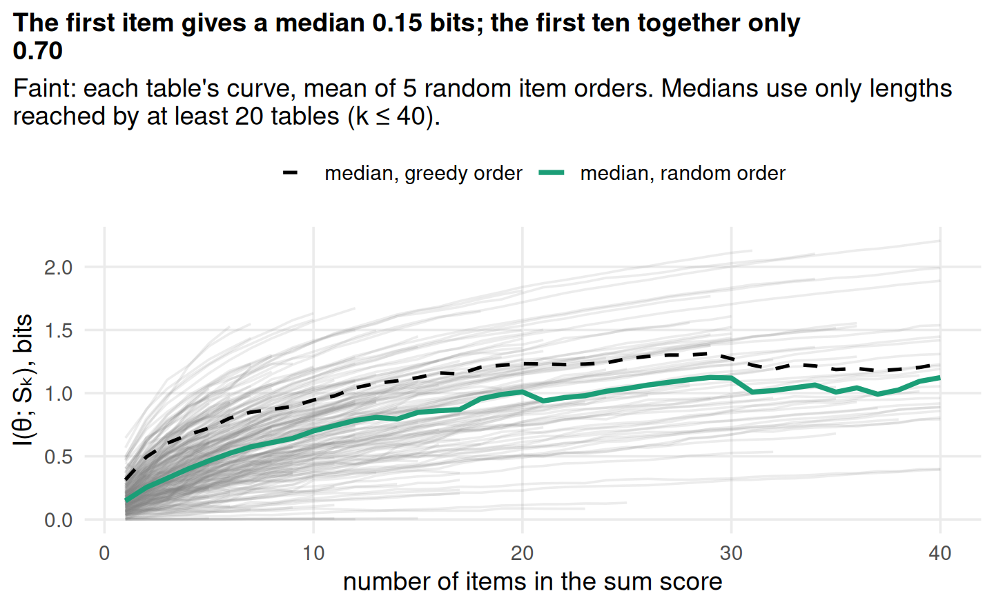
Each additional item adds less than the one before, because it mostly repeats what earlier items already said about the person. The greedy order (best item first, then the item that adds most to it, and so on) shows how much of a test’s information a short form could keep. Among the 104 tables with at least 15 items, the 5 greedy items carry a median 67% of the full sum score’s bits; 5 random items carry 37%.

One curiosity: for a sum score, more items is not always better. Adding a flat item to an unweighted sum adds noise without adding signal, so the curve can turn down. In 38 tables the best five items alone carry more information than the full sum score, up to 3.0 times as much (tuason_2021_covid_coping_enjoy).

Where do the bits come from?

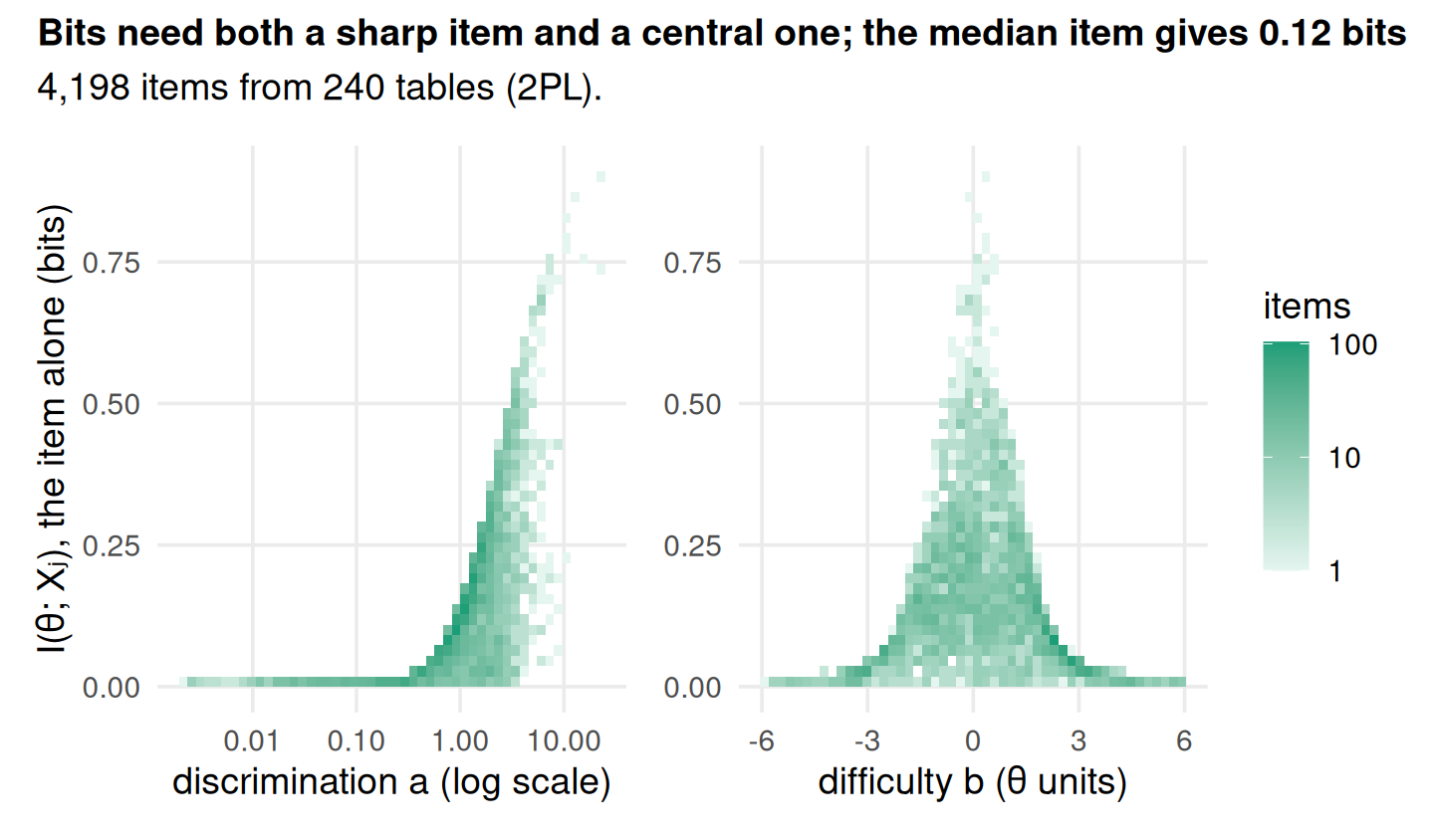
An item’s bits depend on two things. Discrimination is how sharply the item separates people just below its difficulty from people just above. Position is where that cut falls. A highly discriminating item placed far in a tail still says little about most people, because nearly everyone gives the same answer to it. The ceiling is 1 bit, reached only by a perfectly sharp item at the population median.

What does sum-scoring cost?

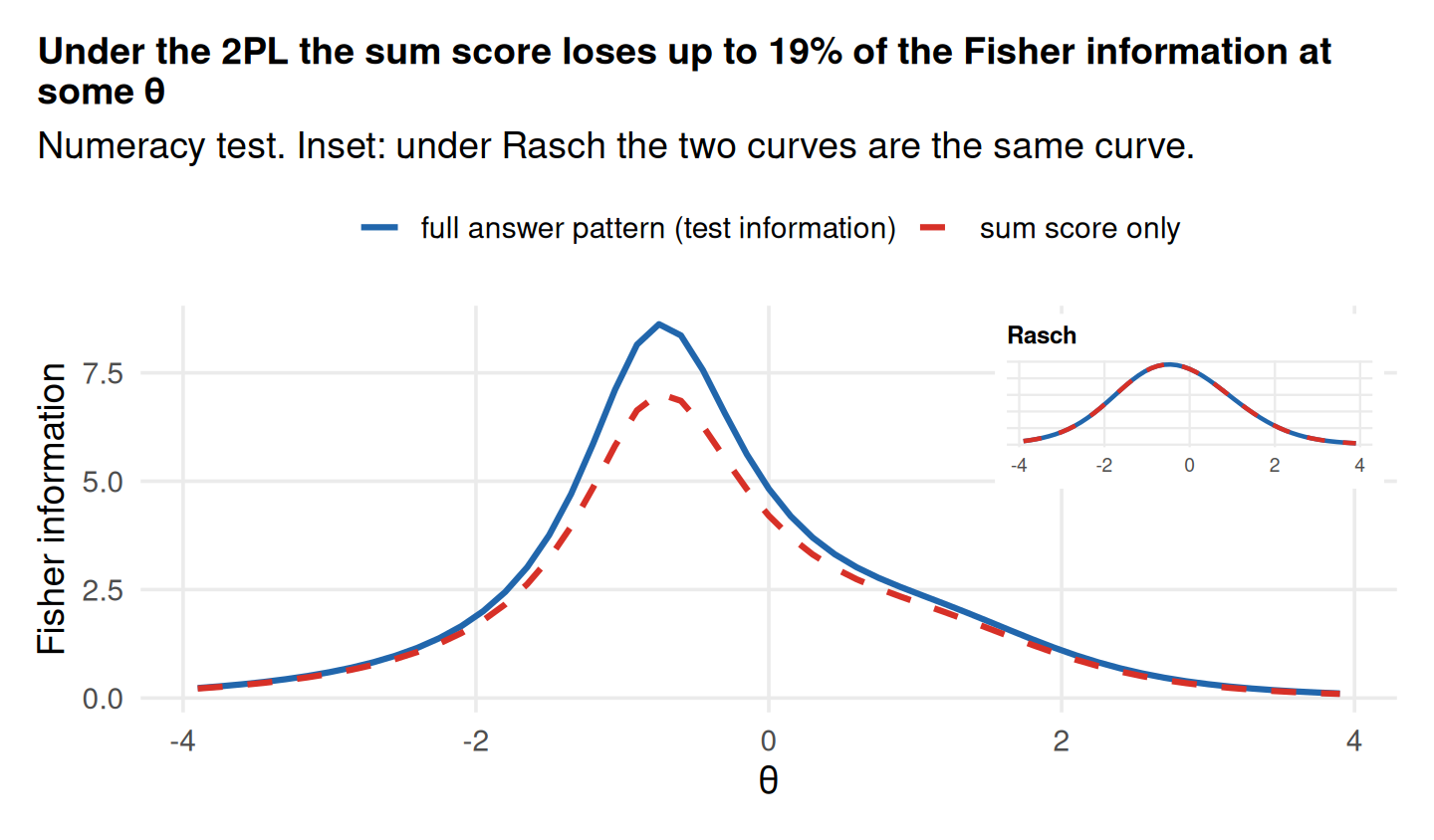
The gap between the full pattern and the sum score has a name: it is the conditional mutual information I(θ; X | S), the information about θ in which items a person got right beyond how many. Under the Rasch model it is zero: the sum score carries every bit the pattern carries. Under the 2PL it is not: with the item parameters known, the sufficient statistic for θ is the slope-weighted score Σj ajXj, which carries every bit the pattern does, I(θ; Σj ajXj) = I(θ; X). The gap is therefore exactly the cost of weighting every item equally when the 2PL says items with higher slopes deserve more weight (Is the sum score enough? takes this further). The loss is small: a median of 7% of the pattern’s information. It exceeds a quarter in 28 tables. As the figure shows, the loss tracks how unequal the slopes are (Spearman correlation 0.87 with the spread of log slopes): tables that mix very sharp items with very flat ones lose the most.

Is the sum score enough?

Every score is computed from the answers, so θ → X → S is a chain: the score can only know what the answers know. That is the data processing inequality, I(θ; S) ≤ I(θ; X). The chain rule splits the full pattern’s information exactly into what the score keeps and what it drops:

I(θ; X) = I(θ; S) + I(θ; X | S).

A statistic is sufficient for θ exactly when nothing is dropped, I(θ; X | S) = 0, whatever the population (Cover and Thomas 2006, sec. 2.9). Equivalently, once you know the score, the rest of the pattern says nothing more about the person. Under the Rasch model the sum score is sufficient; under the 2PL the slope-weighted score Σ ajxj is, and the plain sum is not.

For every population

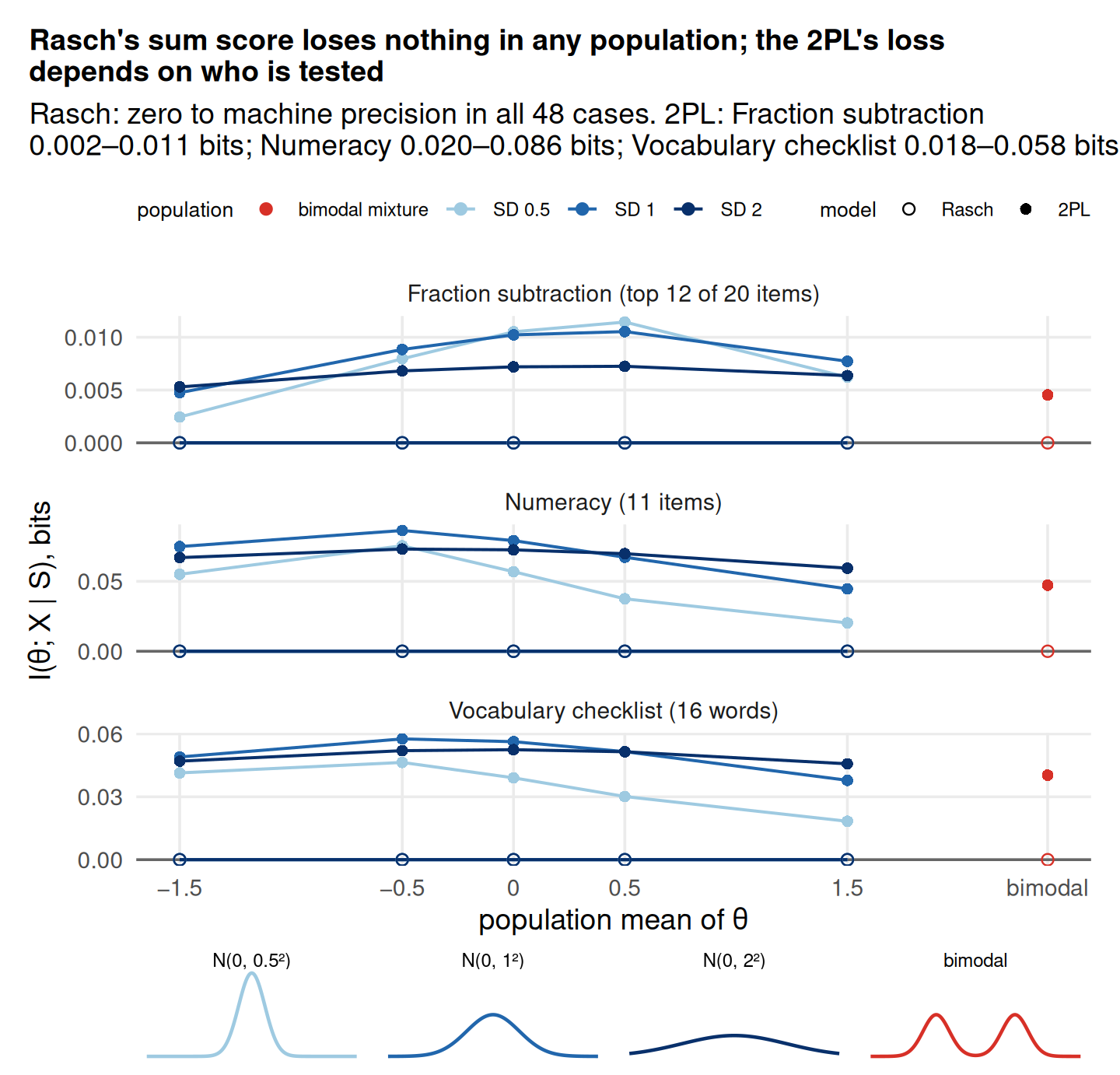
Sufficiency is a statement about every prior, not just the population we happened to sample. To see that, we hold each model’s item parameters fixed and recompute the information under 16 different populations: normal distributions centred anywhere from −1.5 to 1.5 with SDs of 0.5, 1 and 2, plus a two-humped mixture.

The populations matter in two ways. First, the total I(θ; X) changes a lot with the population: a narrow population has less to resolve, and a population far from the items’ difficulties gets mostly uninformative answers. Second, under the 2PL the share of that information hiding in which items were answered moves with it, because which items are informative depends on where people are. Under Rasch none of this touches sufficiency: the gap is zero for every population, as the definition requires.

Compression

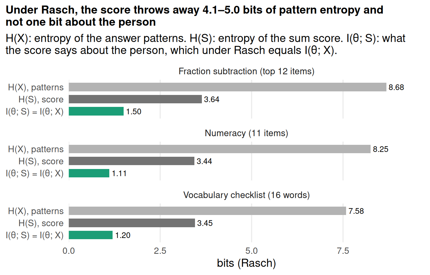
Under Rasch the sum score is a minimal sufficient statistic: it collapses up to 2n patterns into n + 1 scores, the most compression possible without losing anything about θ. For the numeracy test that is 2,048 patterns into 12 scores. In bits, the patterns carry 8.25 bits of entropy, the score 3.44, and both carry the same 1.110 bits about the person. Everything else the patterns say is noise as far as θ is concerned. That last step is special to Rasch. Under the 2PL the sum score is no longer sufficient, and the same compression costs some bits about the person (a median of 7% across the warehouse, from What does sum-scoring cost?); the compression that loses nothing is to the slope-weighted score instead.

Same score, different patterns

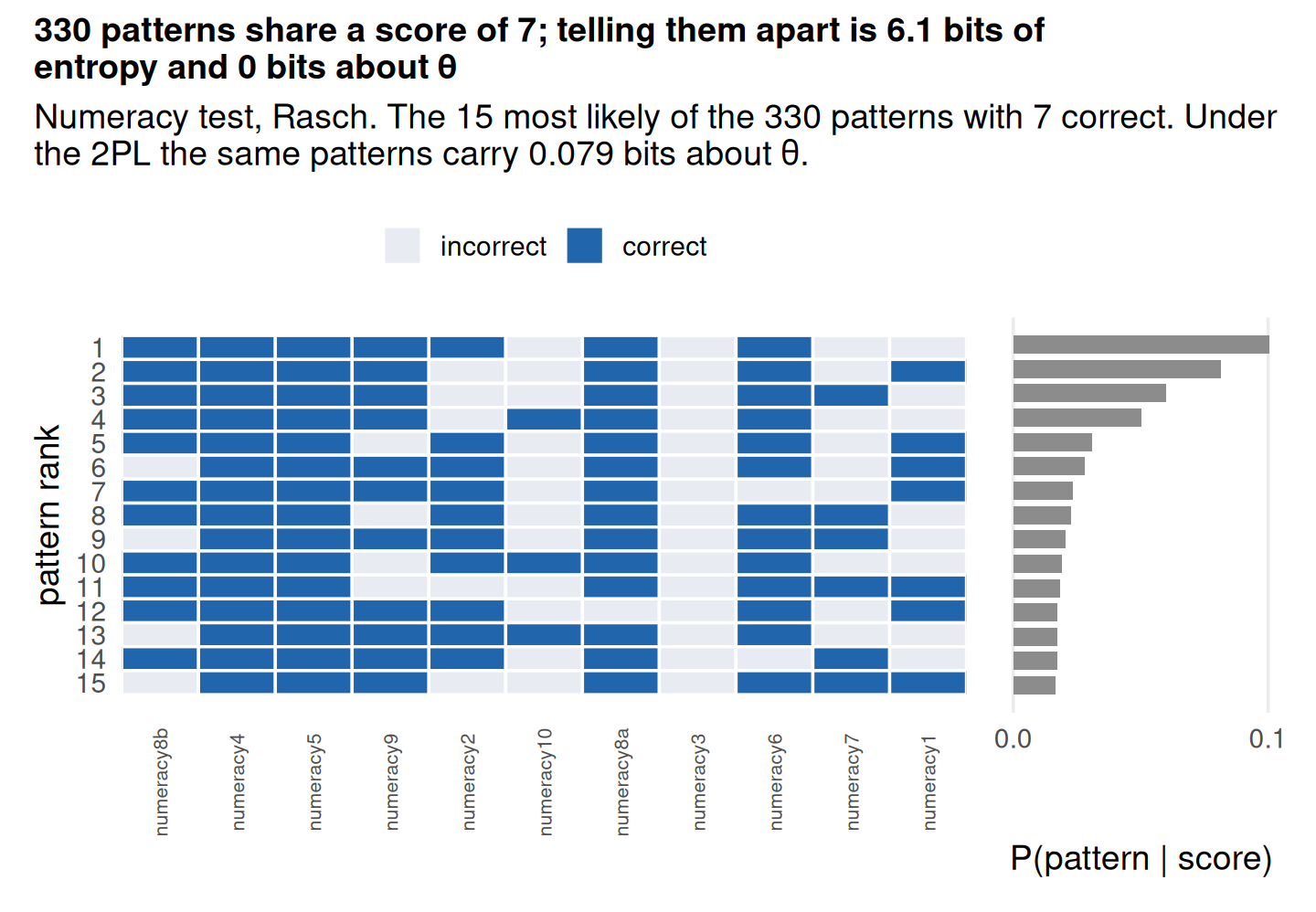
Many patterns share each score: under Rasch, H(X | S = 7) is 6.10 bits. Yet I(θ; X | S = 7) is zero, because the probability of each pattern given its score does not depend on θ at all. Two people with the same score but very different θ produce these patterns in exactly the same proportions. This θ-free conditional distribution is what conditional maximum likelihood estimates item parameters from.

Where misfit lives

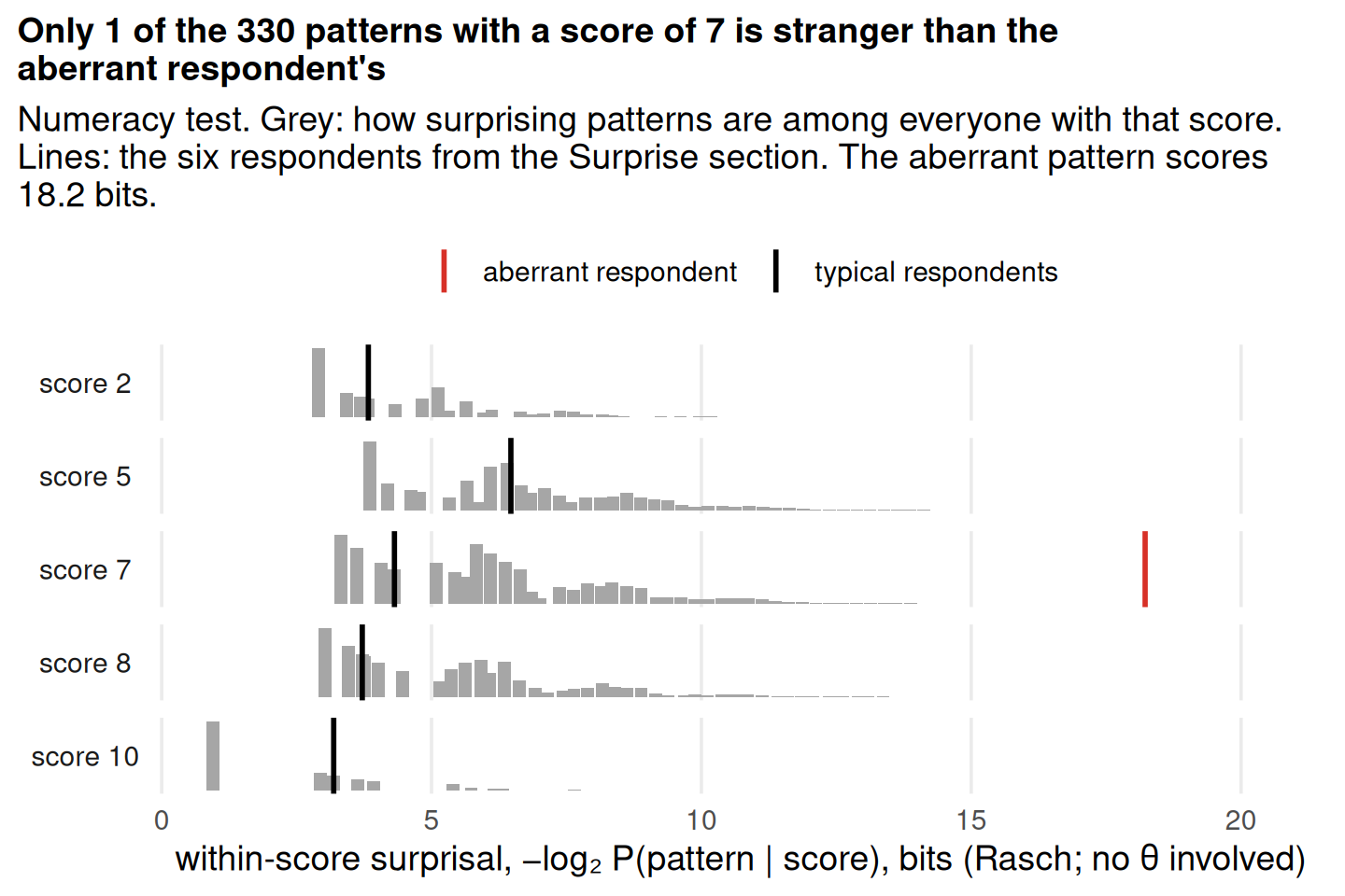
The θ-free part of the data is where fit lives. A pattern can be very surprising given its score while saying nothing about the person’s level. This is a different surprisal from the one in the Surprise section, which asked how unexpected each answer was given where the person’s other answers placed them on θ. Here θ never enters. The question is only whether this arrangement of correct answers is a plausible one for someone with this many correct answers. Recall the aberrant respondent from the Surprise section: the person with the worst person-fit in the numeracy data (Zh = -5.8), who misses 2 of the 3 easiest questions yet gets 3 of the 3 hardest right. By this measure their pattern is among the least plausible at their score: right on hard items, wrong on easy ones, the reverse of what the score leads you to expect.

The Fisher view

Two classical facts say the same thing in other units. A sufficient statistic preserves the Kullback–Leibler divergence between the response distributions of any two values of θ, so any two people are exactly as distinguishable from their score as from their full patterns. And it preserves Fisher information at every θ, so the score’s test information function equals the full data’s. Under the 2PL the plain sum score loses a little of both, and the slope-weighted score keeps both (Cover and Thomas 2006).

From groups to continuous θ

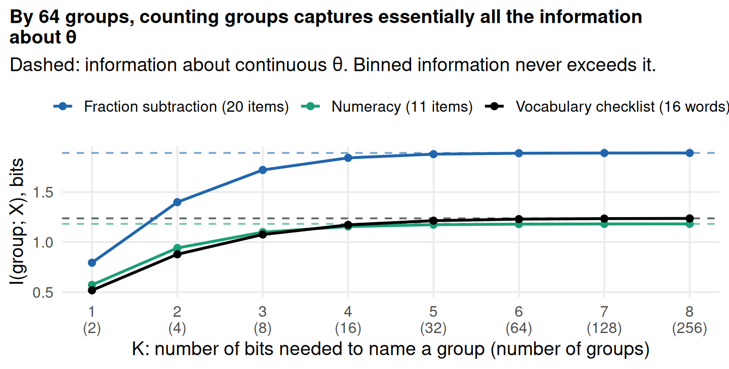
The game above asks “which of 64 groups?”. The warehouse numbers ask about θ itself, a continuous quantity. These are close: information about the group can never exceed information about θ, since knowing θ tells you the group, and it converges to it as the groups get finer. With 2 groups the numeracy test gives 0.57 bits. With 64 it gives 1.179, against 1.182 for continuous θ. Because the tests deliver only one or two bits, six bits of groups is far more resolution than any of them can use.

More than right and wrong

Many tables in the warehouse do not record right and wrong answers. They record a choice among ordered categories: strongly disagree to strongly agree, not at all to nearly every day. Everything above carries over to such items. Two things are new: the ceiling on what one item can deliver, and a question that right-or-wrong items never raise, how many categories an item needs. Rather than the whole warehouse, this section works through three familiar instruments under the generalized partial credit model (GPCM), the polytomous counterpart of the 2PL.

The three are the Rosenberg self-esteem scale (Rosenberg 1965) (10 statements, four categories from strongly disagree to strongly agree), the ten extraversion items of a Big Five inventory (five categories), and the GAD-7 anxiety screener (seven symptoms, from not at all to nearly every day over the last two weeks). Each was subsampled to 10,000 respondents. Half the Rosenberg and extraversion items are worded against the trait (“I certainly feel useless at times”, “I keep in the background”), and the warehouse stores them as answered; we reversed them before fitting (Rosenberg items 3, 5, 8, 9, 10; extraversion E2, E4, E6, E8, E10). Reversal changes nothing about how many bits an item carries; it only makes a higher category mean more of the trait on every item.

One item, four bins

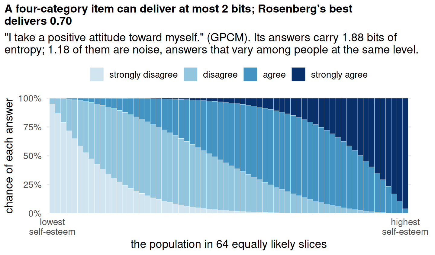
A right-or-wrong item asks one yes/no question, so it can deliver at most 1 bit. Four categories sort people into four bins, which is the three-cut case from the opening widget. Telling four equally full bins apart takes two yes/no questions (upper half or lower half? then upper or lower within it?), so the ceiling is 2 bits. In general it is log2 K: 1.58 bits for three categories, 2.32 for five. The ceiling is reached only by an item whose categories are perfectly sharp and equally full. The decomposition is the one used throughout, I(θ; Xj) = H(Xj) − H(Xj | θ). The only difference is that the noise term is now a category entropy, −Σk Pk(θ) log2 Pk(θ), averaged over the population. The figure shows why it is large. Even among the most self-assured slice of people, the statement draws a mix of agree and strongly agree, and that mix is noise as far as θ is concerned.

Some of that noise is not luck. People differ in how they use a response scale: some favour the extremes, others the midpoint, whatever their level of the trait. A one-dimensional model has nowhere to put those response styles except H(Xj | θ). The answers carry information about something, but not about θ.

Categories offered, categories used

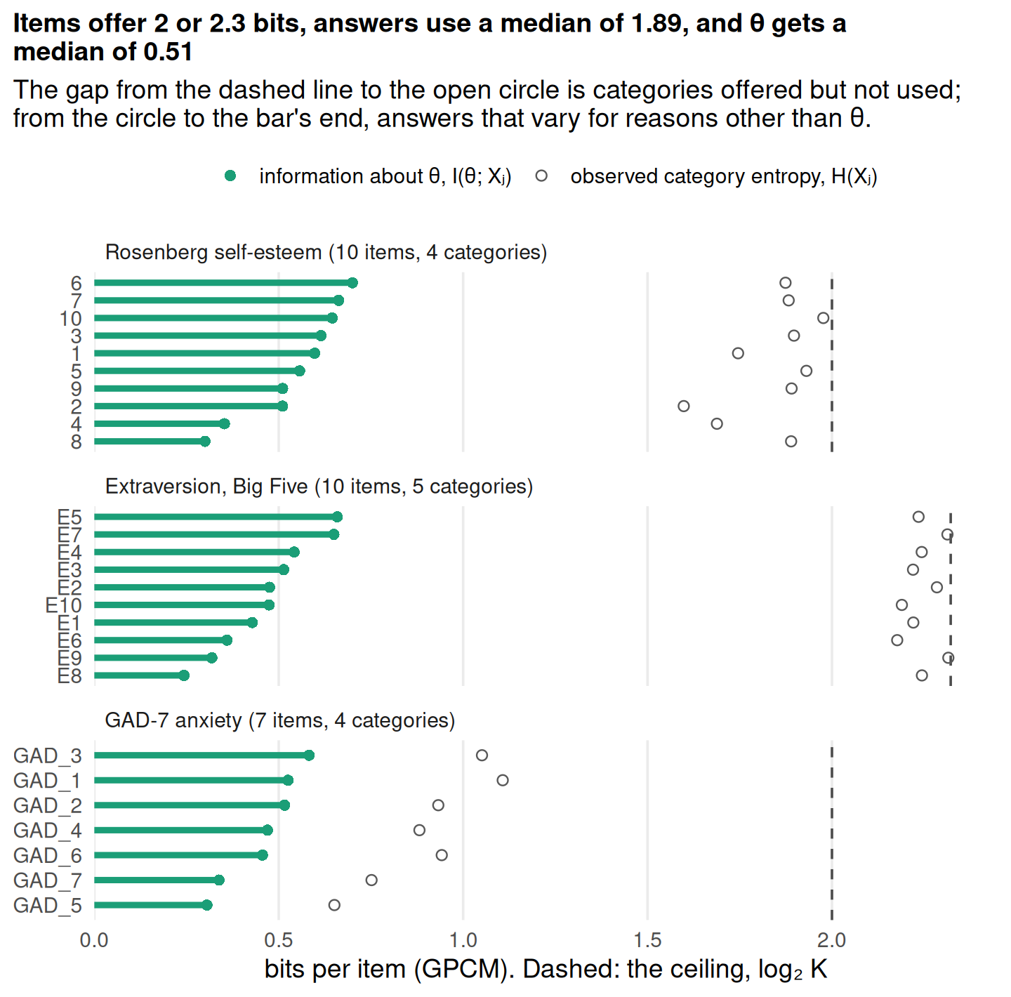
The label on the scale sets the ceiling, log2 K. A tighter ceiling comes from the data: the entropy of the answers actually given, H(Xj). If respondents use only two of an item’s five categories, the item cannot deliver much more than 1 bit, whatever its label. The GAD-7 makes the point. Its four categories offer 2 bits per item, but in this general-population sample 97%–99% of people answer each item not at all or several days, so the answers carry only 0.65–1.11 bits of entropy, and θ gets 0.31–0.58 of them. The extraversion items use nearly all of their 2.32 bits (2.18–2.32), yet deliver only 0.24–0.66 bits about θ. Their categories are all in use; most of that use is noise. Across the three tables a single polytomous item delivers a median of 0.51 bits, against a median of 0.12 for a dichotomous item in the warehouse. That is more than one right-or-wrong question, and a long way below the ceiling.

How many categories do you need?

Merging adjacent categories (counting agree and strongly agree as one answer, say) is a function of the response, so by the data processing inequality it can only lose information. The chain rule says exactly how much: the loss is I(θ; Xj | merged Xj), the information in the distinction the merge erases. A four-category item has seven ways to merge adjacent categories and a five-category item fifteen. We evaluated each under the fitted model, without refitting.

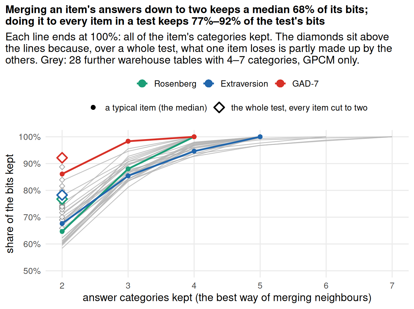
The answer depends on the item. For “I wish I could have more respect for myself.” the best two-way split keeps 70% of the item’s bits. For “I feel that I am a person of worth, at least on an equal plane with others.” it keeps 58%.

Over a whole test the losses are smaller, because the items overlap. Taken one at a time, Rosenberg’s ten items carry 5.45 bits between them, but the test as a whole carries only 1.82: most of what each item says, the other nine already say. So when a merge erases a fine distinction on one item (agree against strongly agree, say), the other items have already placed the person roughly, and the lost distinction would mostly have repeated them. Merging every Rosenberg item down to two keeps 77% of the test’s bits, against 65% for a typical item on its own. Dichotomizing every GAD-7 item at its best split (in practice, not at all against everything else) keeps 92% of the test’s 1.24 bits. That is the “categories offered are not categories used” point, put in bits: almost all of the GAD-7’s information is in whether a symptom is present at all. Extraversion, whose categories are all in use, keeps 78%. The grey lines are a random draw of 27 further warehouse tables with 4–7 categories (GPCM only, no reverse keying, which mutual information ignores). They tell the same story: cutting a typical item to two keeps 58%–84% of its bits, three categories keep a median 87%, and cutting every item in a test to two keeps 66%–89% of the test’s bits.

The scatter puts the same losses on the absolute scale (dashed line: nothing lost; solid grey: the median share; hover over a dot for the table; larger dots are longer tests). The gap to the dashed line is I(θ; X | dichotomised X), the information in the merged distinctions that the other items do not already repeat. It grows with the test’s total, roughly in proportion, so no table loses more than about a third of its bits and no table escapes the loss.

The three tests under the GPCM. Share of Σ log₂ K: I(θ; X) as a share of the most the items could deliver. −½ log₂(1 − ρ): the Gaussian bits implied by marginal reliability. Dichotomized: I(θ; X) with every item cut at its best split.
Test I(θ; X) bits per item share of Σ log₂ K −½ log₂(1 − ρ) dichotomized
Rosenberg self-esteem (10 items, 4 categories) 1.82 0.18 9% 1.77 1.40
Extraversion, Big Five (10 items, 5 categories) 1.67 0.17 7% 1.62 1.31
GAD-7 anxiety (7 items, 4 categories) 1.24 0.18 9% 0.78 1.14

Limitations

  • Model dependence. Every number is computed from a fitted model, not from the data directly. If a 2PL is wrong for a table (guessing, multiple dimensions, local dependence), the bits are wrong too. The sum-score check gives one warning sign: model-implied and observed score distributions diverge by more than 0.1 bit (KL) in 37 tables.
  • Local dependence and sharp items. Even with a slope prior, 34 tables have at least one item with a slope above 5, often near-duplicate items. Such pairs make the model treat a repeated answer as two independent pieces of evidence, which inflates the bits.
  • Unidimensionality. We fit one trait per table. A multidimensional test carries information about several traits, and the numbers here count only what projects onto the first.
  • The population matters. Information is relative to the spread of people taking the test. The same items given to a more homogeneous group would deliver fewer bits, because there is less uncertainty to resolve to begin with.
  • Subsampling and missing data. Large tables were subsampled to 10,000 respondents; that affects parameter precision, not the definition of the quantity. Items answered by fewer than half the respondents were dropped, and I(θ; X) treats every respondent as answering every remaining item.
  • Convergence. 1 2PL fit (onah_2021_covid_info_sources) did not meet mirt’s convergence criterion; its results are included but should be read with care.
  • Enumeration in the sufficiency section. Its quantities enumerate every answer pattern on a θ grid, so they are limited to 16 items. For the fraction-subtraction test they use the 12 items with the highest expected bits. The within-score surprisal needs no θ grid and uses all items.
  • Scope. The warehouse-wide numbers cover only dichotomous items, and no ENEM tables in this version. The polytomous section uses three tables, chosen by hand, not a sample of the warehouse’s polytomous tables.
  • Polytomous models and choices. The polytomous bits depend on the model as much as the dichotomous ones do. The section reports the generalized partial credit model; under the partial credit and graded response models a test’s bits change by up to 0.12 bits. Negatively worded items were reversed before fitting. Every category was kept, including GAD-7’s sparse top category (nearly every day, under 1.5% of answers on every item), which leaves its estimates the least precise. Merged categories were evaluated under the model fitted to the full categories, without refitting. That isolates what the distinction is worth under one model, but a model refitted to the merged data could tell a slightly different story. 9 of 9 polytomous fits converged. Rosenberg and the GAD-7 were enumerated exactly (up to 410 = 1,048,576 patterns); extraversion (510 patterns) used Monte Carlo (standard error under 0.005 bits).

Reproducibility

Source code for this page: bits_per_item.qmd · bits_per_item_checks.R · bits_per_item_compute.R · bits_per_item_helpers.R · bits_per_item_poly_compute.R · bits_per_item_poly_extra.R · bits_per_item_poly_helpers.R · bits_per_item_poly_scout.R · bits_per_item_reliability_sim.R · bits_per_item_scout.R · bits_per_item_sufficiency.R

These results were computed against approximately IRW v568 (the corpus as of October 13, 2026).

The version was inferred from when the results were computed, not recorded during the run, so it may be off by a version or more. 2 IRW versions were released that day, so the exact one is ambiguous. To pin data to an exact version, use irw_use_version().

Results were computed on October 05, 2026. To regenerate:

# 0. Optional: re-scan IRW for eligible tables (writes scout_tables.csv)
source("vignettes/bits_per_item_scout.R")

# 1. Validation checks, then the compute script (from the project root)
source("vignettes/bits_per_item_checks.R")
source("vignettes/bits_per_item_compute.R")

# 1b. The polytomous section (three tables; checks are the "P" block above)
source("vignettes/bits_per_item_poly_compute.R")

# 2. Re-render this page
quarto::quarto_render("vignettes/bits_per_item.qmd")
Tip

To cite the datasets used, run:

irw_save_bibtex(unique(summary_df$table), output_file = "bits_per_item_data/references.bib")

Visual inspiration: 3Blue1Brown, “Solving Wordle using information theory”. No material from the video is reused here.


References

n.d.-a. In LDbase. Florida State University Libraries. https://doi.org/10.33009/ldbase.1624481381.d9ec.
n.d.-b. In LDbase. Florida State University Libraries. https://doi.org/10.33009/ldbase.1680213217.8ed0.
n.d.-c. In LDbase. Florida State University Libraries. https://doi.org/10.33009/ldbase.1620837890.bcf8.
Abaluck, Jason, Laura H. Kwong, Ashley Styczynski, et al. 2022. “Impact of Community Masking on COVID-19: A Cluster-Randomized Trial in Bangladesh.” Science 375 (6577). https://doi.org/10.1126/science.abi9069.
“Actitudes de La Juventud En España Hacia La Participación y El Voluntariado.” 2024. Centro de Investigaciones Sociológicas. https://www.cis.es/es/estudios/actitudes-de-la-juventud-en-espana-hacia-la-participacion-y-el-voluntariado?cuestionario=16911&muestra=22473&pregunta=537787&variable=613925&chartType=bar.
Alsuhibani, Azzam, Mark Shevlin, Daniel Freeman, Bryony Sheaves, and Richard P. Bentall. 2022. “Why Conspiracy Theorists Are Not Always Paranoid: Conspiracy Theories and Paranoia Form Separate Factors with Distinct Psychological Predictors.” PLOS ONE 17 (4): e0259053. https://doi.org/10.1371/journal.pone.0259053.
Altgassen, Elisa, Catherine Schittenhelm, and Oliver Wilhelm. 2025a. “Words Don’t Come Easy: How Lexical Difficulty of Items and Vocabulary of Subjects (Not) Affect Personality Assessment.” Journal of Personality and Social Psychology 129 (5): 910–32. https://doi.org/10.1037/pspp0000572.
Altgassen, Elisa, Catherine Schittenhelm, and Oliver Wilhelm. 2025b. “Words Don’t Come Easy: How Lexical Difficulty of Items and Vocabulary of Subjects (Not) Affect Personality Assessment.” Journal of Personality and Social Psychology 129 (5): 910–32. https://doi.org/10.1037/pspp0000572.
Andersen, Erling B. 1977. “Sufficient Statistics and Latent Trait Models.” Psychometrika 42 (1): 69–81. https://doi.org/10.1007/BF02293746.
Anunciacao, Luis, Christopher Murray, Kimberly Murphy, and Jane Squires. 2026. “Socio-Emotional Profiles of Young Children with and Without Developmental Delay.” International Journal of Early Childhood, ahead of print, March. https://doi.org/10.1007/s13158-026-00488-y.
Anunciação, Luis, Louise Marques, Christopher Murray, et al. 2024. “Psychometric Properties of a Brief Non-Verbal Test of g Factor Intelligence.” Journal of Psychological Perspective 6 (1): 47–62. https://doi.org/10.47679/jopp.617532024.
Arteaga, Irma, Andreas de Barros, and Alejandro J. Ganimian. 2025a. “The Challenges of Scaling up Effective Child-Rearing Practices Using Technology in Developing Settings: Experimental Evidence from India.” Journal of Research on Educational Effectiveness, March, 1–19. https://doi.org/10.1080/19345747.2025.2450318.
Arteaga, Irma, Andreas de Barros, and Alejandro J. Ganimian. 2025b. “The Challenges of Scaling up Effective Child-Rearing Practices Using Technology in Developing Settings: Experimental Evidence from India.” Journal of Research on Educational Effectiveness, March, 1–19. https://doi.org/10.1080/19345747.2025.2450318.
Banerjee, Abhijit, Rukmini Banerji, Esther Duflo, et al. 2017a. Raw and Replication Data for: ’From Proof of Concept to Scalable Policies’ and ’Mainstreaming an Effective Intervention’. Harvard Dataverse. https://doi.org/10.7910/DVN/DUBA3J.
Banerjee, Abhijit, Rukmini Banerji, Esther Duflo, et al. 2017b. Raw and Replication Data for: ’From Proof of Concept to Scalable Policies’ and ’Mainstreaming an Effective Intervention’. Harvard Dataverse. https://doi.org/10.7910/DVN/DUBA3J.
Banerjee, Abhijit, Rukmini Banerji, Esther Duflo, et al. 2017c. Raw and Replication Data for: ’From Proof of Concept to Scalable Policies’ and ’Mainstreaming an Effective Intervention’. Harvard Dataverse. https://doi.org/10.7910/DVN/DUBA3J.
Banerjee, Abhijit, Rukmini Banerji, Esther Duflo, et al. 2017d. Raw and Replication Data for: ’From Proof of Concept to Scalable Policies’ and ’Mainstreaming an Effective Intervention’. Harvard Dataverse. https://doi.org/10.7910/DVN/DUBA3J.
Banerji, Rukmini, James Berry, and Marc Shotland. 2017a. The Impact of Maternal Literacy and Participation Programs: Evidence from a Randomized Evaluation in India. Harvard Dataverse. https://doi.org/10.7910/DVN/19PPE7.
Banerji, Rukmini, James Berry, and Marc Shotland. 2017b. The Impact of Maternal Literacy and Participation Programs: Evidence from a Randomized Evaluation in India. Harvard Dataverse. https://doi.org/10.7910/DVN/19PPE7.
Bartholomew, D. J. 1998. “Scaling Unobservable Constructs in Social Science.” Journal of the Royal Statistical Society Series C: Applied Statistics 47 (1): 1–13. https://doi.org/10.1111/1467-9876.00094.
Bartoli, Nicola, and Simone Benedetto. 2022. “Driven by Notifications – Exploring the Effects of Badge Notifications on User Experience.” PLOS ONE 17 (6): e0270888. https://doi.org/10.1371/journal.pone.0270888.
Bartolucci, Francesco, Silvia Bacci, and Michela Gnaldi. 2014. “MultiLCIRT: An r Package for Multidimensional Latent Class Item Response Models.” Computational Statistics &Amp; Data Analysis 71 (March): 971–85. https://doi.org/10.1016/j.csda.2013.05.018.
Bentall, Richard, Mark Shevlin, Orla McBride, et al. 2022a. The COVID-19 Psychological Research Consortium Study, 2020-2021. UK Data Service. https://doi.org/10.5255/UKDA-SN-855552.
Bentall, Richard, Mark Shevlin, Orla McBride, et al. 2022b. The COVID-19 Psychological Research Consortium Study, 2020-2021. UK Data Service. https://doi.org/10.5255/UKDA-SN-855552.
Bentall, Richard, Mark Shevlin, Orla McBride, et al. 2022c. The COVID-19 Psychological Research Consortium Study, 2020-2021. UK Data Service. https://doi.org/10.5255/UKDA-SN-855552.
Bentall, Richard, Mark Shevlin, Orla McBride, et al. 2022d. The COVID-19 Psychological Research Consortium Study, 2020-2021. UK Data Service. https://doi.org/10.5255/UKDA-SN-855552.
Berry, James, Hyuncheol Bryant Kim, and Hyuk Harry Son. 2021a. Replication Data for: When Student Incentives Don’t Work: Evidence from a Field Experiment in Malawi. Harvard Dataverse. https://doi.org/10.7910/DVN/FXL7JW.
Berry, James, Hyuncheol Bryant Kim, and Hyuk Harry Son. 2021b. Replication Data for: When Student Incentives Don’t Work: Evidence from a Field Experiment in Malawi. Harvard Dataverse. https://doi.org/10.7910/DVN/FXL7JW.
Bialowolski, Piotr. 2024. Financial Literacy in a Gendered Language Context. Harvard Dataverse. https://doi.org/10.7910/DVN/MTQGSF.
Bitew, Tesera, Wohabie Birhan, and Demeke Wolie. 2020. “Perceived Learning Difficulty Associates with Depressive Symptoms and Substance Use Among Students of Higher Educational Institutions in North Western Ethiopia: A Cross Sectional Study.” PLOS ONE 15 (11): e0240914. https://doi.org/10.1371/journal.pone.0240914.
Bock, R. Darrell, and Marcus Lieberman. 1970. “Fitting a Response Model for n Dichotomously Scored Items.” Psychometrika 35 (2): 179–97. https://doi.org/10.1007/bf02291262.
Bohn, Manuel, Julia Christin Prein, Tobias Koch, et al. 2022. oREV: An Item Response Theory Based Open Receptive Vocabulary Task for 3 to 8-Year-Old Children. August. https://doi.org/10.31234/osf.io/4z86w.
Brennan, K., C. Clark, and P. Shaver. 2014. Roseberg Self-Esteem Scale [Dataset and Codebook]. http://openpsychometrics.org/_rawdata/RSE.zip.
Brotherton, Robert, Christopher C. French, and Alan D. Pickering. 2013. “Measuring Belief in Conspiracy Theories: The Generic Conspiracist Beliefs Scale.” Frontiers in Psychology 4. https://doi.org/10.3389/fpsyg.2013.00279.
Bruhn, Miriam, Luciana De Souza Leão, Arianna Legovini, Rogelio Marchetti, and Bilal Zia. 2016. Replication Data for: The Impact of High School Financial Education: Evidence from a Large-Scale Evaluation in Brazil. ICPSR - Interuniversity Consortium for Political; Social Research. https://doi.org/10.3886/E116339V1.
Buchanan, Erin Michelle, Riley E. Foreman, Becca Nicole Huber, Jeffrey Michael Pavlacic, Rachel N. Swadley, and Stefan E. Schulenberg. 2017. Does the Delivery Matter? Examining Randomization at the Item Level. November. https://doi.org/10.31219/osf.io/p93df.
Busch, Carly A., Katelyn M. Cooper, and Sara E. Brownell. 2023. “Women Drive Efforts to Highlight Concealable Stigmatized Identities in u.s. Academic Science and Engineering.” PLOS ONE 18 (7): e0287795. https://doi.org/10.1371/journal.pone.0287795.
Busch, Carly A., Tasneem F. Mohammed, Erika M. Nadile, and Katelyn M. Cooper. 2022a. “Aspects of Online College Science Courses That Alleviate and Exacerbate Undergraduate Depression.” PLOS ONE 17 (6): e0269201. https://doi.org/10.1371/journal.pone.0269201.
Busch, Carly A., Tasneem F. Mohammed, Erika M. Nadile, and Katelyn M. Cooper. 2022b. “Aspects of Online College Science Courses That Alleviate and Exacerbate Undergraduate Depression.” PLOS ONE 17 (6): e0269201. https://doi.org/10.1371/journal.pone.0269201.
Bužgová, Radka, Radka Kozáková, Katka Bobčíková, and Renáta Zeleníková. 2023a. “Predictors of Life Satisfaction in Elders Living at Home in the Czech Republic.” PLOS ONE 18 (3): e0283772. https://doi.org/10.1371/journal.pone.0283772.
Bužgová, Radka, Radka Kozáková, Katka Bobčíková, and Renáta Zeleníková. 2023b. “Predictors of Life Satisfaction in Elders Living at Home in the Czech Republic.” PLOS ONE 18 (3): e0283772. https://doi.org/10.1371/journal.pone.0283772.
Cabell, Sonia Q., James S. Kim, Thomas G. White, et al. 2025a. “Impact of a Content-Rich Literacy Curriculum on Kindergarteners’ Vocabulary, Listening Comprehension, and Content Knowledge.” Journal of Educational Psychology 117 (2): 153–75. https://doi.org/10.1037/edu0000916.
Cabell, Sonia Q., James S. Kim, Thomas G. White, et al. 2025b. “Impact of a Content-Rich Literacy Curriculum on Kindergarteners’ Vocabulary, Listening Comprehension, and Content Knowledge.” Journal of Educational Psychology 117 (2): 153–75. https://doi.org/10.1037/edu0000916.
Centro de Investigaciones Sociológicas. 2023. “Ciudadanía (ISSP).” No. 3020. Centro de Investigaciones Sociológicas. https://www.cis.es/es/estudios/ciudadania-issp-?cuestionario=16860&muestra=22521&pregunta=541045&variable=630618&chartType=bar.
Centro de Investigaciones Sociológicas. 2024. “Opiniones y Actitudes Ante La Unión Europea (II).” No. 3523. Centro de Investigaciones Sociológicas. https://www.cis.es/es/estudios/opiniones-y-actitudes-ante-la-union-europea-ii-?cuestionario=17976&muestra=26298&pregunta=655316&variable=1083448&chartType=bar.
Centro de Investigaciones Sociológicas (CIS). 2012a. “Percepción Social de La Violencia de Género.” No. 2968. Centro de Investigaciones Sociológicas. https://www.cis.es/es/estudios/percepcion-social-de-la-violencia-de-genero?chartType=bar&cuestionario=16887&muestra=22437&pregunta=534829&variable=597302.
Centro de Investigaciones Sociológicas (CIS). 2012b. “Percepción Social de La Violencia de Género.” No. 2968. Centro de Investigaciones Sociológicas. https://www.cis.es/es/estudios/percepcion-social-de-la-violencia-de-genero?chartType=bar&cuestionario=16887&muestra=22437&pregunta=534829&variable=597302.
Centro de Investigaciones Sociológicas (CIS). 2015. Calidad de Los Servicios Públicos VIII. Centro de Investigaciones Sociológicas; CIS. https://www.cis.es/es/estudios/calidad-de-los-servicios-publicos-viii-?chartType=bar&cuestionario=16908&muestra=22449&pregunta=536716&variable=603732.
Centro de Investigaciones Sociológicas (CIS). 2023. “Debate Sobre El Estado de La Nación (XXIV).” No. 3016. https://www.cis.es/es/estudios/debate-sobre-el-estado-de-la-nacion-xxiv-?cuestionario=16848\&muestra=22410\&pregunta=532810.
Centro de Investigaciones Sociológicas (CIS). 2024a. “Barómetro de La Vivienda y El Alquiler.” No. 3212. Centro de Investigaciones Sociológicas. https://www.cis.es/es/estudios/barometro-de-la-vivienda-y-el-alquiler?cuestionario=17329&muestra=24021&pregunta=592252&variable=807645&chartType=bar.
Centro de Investigaciones Sociológicas (CIS). 2024b. “Barómetro de La Vivienda y El Alquiler.” No. 3212. https://www.cis.es/es/estudios/barometro-de-la-vivienda-y-el-alquiler?cuestionario=17329&muestra=24021&pregunta=592252&variable=807645&chartType=bar.
Centro de Investigaciones Sociológicas (CIS). 2024c. “Debate Sobre El Estado de La Nación (XXIV).” No. 3016. Centro de Investigaciones Sociológicas. https://www.cis.es/es/estudios/debate-sobre-el-estado-de-la-nacion-xxiv-?cuestionario=16848&muestra=22410&pregunta=532810.
Centro de Investigaciones Sociológicas (CIS). 2024d. “Inteligencia Artificial, Estudio 3495.” https://www.cis.es/es/estudios/inteligencia-artificial?chartType=bar&cuestionario=17941&muestra=26186&pregunta=653660&variable=1073709.
Centro de Investigaciones Sociológicas (CIS). 2024e. “Inteligencia Artificial.” No. 3495. https://www.cis.es/es/estudios/inteligencia-artificial?chartType=bar&cuestionario=17941&muestra=26186&pregunta=653660&variable=1073709.
Centro de Investigaciones Sociológicas (CIS). n.d.-a. “Actitudes de La Juventud En España Hacia El Emprendimiento.” No. 2938. Centro de Investigaciones Sociológicas. https://www.cis.es/es/estudios/actitudes-de-la-juventud-en-espana-hacia-el-emprendimiento?chartType=bar&cuestionario=16438&muestra=21859&pregunta=529937&variable=557680.
Centro de Investigaciones Sociológicas (CIS). n.d.-b. “Actitudes Hacia La Inmigración (VIII).” No. 3119. Centro de Investigaciones Sociológicas. https://www.cis.es/es/estudios/actitudes-hacia-la-inmigracion-viii-?cuestionario=17109&muestra=22655&pregunta=557428&variable=670823&chartType=bar.
Centro de Investigaciones Sociológicas (CIS). n.d.-c. “La Defensa Nacional y Las Fuerzas Armadas (x).” No. 2998. Estudio. https://www.cis.es/es/estudios/la-defensa-nacional-y-las-fuerzas-armadas-x-?cuestionario=16525&muestra=21866&pregunta=269269&variable=559566&chartType=bar.
Centro de Investigaciones Sociológicas (CIS). n.d.-d. “Opiniones y Actitudes Ante La Unión Europea (II).” No. 3523. https://www.cis.es/es/estudios/opiniones-y-actitudes-ante-la-union-europea-ii-?cuestionario=17976&muestra=26298&pregunta=655316&variable=1083448&chartType=bar.
Centro de Investigaciones Sociológicas (CIS). n.d.-e. “Opiniones y Actitudes Sobre La Familia (II).” No. 3032. https://www.cis.es/es/estudios/opiniones-y-actitudes-sobre-la-familia-ii-?cuestionario=16893&muestra=22465&pregunta=536541&variable=604458&chartType=bar.
Christensen, Alexander P., Yoed N. Kenett, Tomaso Aste, Paul J. Silvia, and Thomas R. Kwapil. 2018a. “Network Structure of the Wisconsin Schizotypy Scales–Short Forms: Examining Psychometric Network Filtering Approaches.” Behavior Research Methods 50 (6): 2531–50. https://doi.org/10.3758/s13428-018-1032-9.
Christensen, Alexander P., Yoed N. Kenett, Tomaso Aste, Paul J. Silvia, and Thomas R. Kwapil. 2018b. “Network Structure of the Wisconsin Schizotypy Scales–Short Forms: Examining Psychometric Network Filtering Approaches.” Behavior Research Methods 50 (6): 2531–50. https://doi.org/10.3758/s13428-018-1032-9.
Christie, Richard, and Florence L. Geis. 1970. Studies in Machiavellianism. Academic Press. https://openpsychometrics.org/_rawdata/.
Cohen, Isabelle ; Abubakar, Maryam ; Perlman, Daniel. 2023a. Pathways to Choice: A Bundled Intervention Against Child Marriage. https://doi.org/10.26085/C31C71.
Cohen, Isabelle ; Abubakar, Maryam ; Perlman, Daniel. 2023b. Pathways to Choice: A Bundled Intervention Against Child Marriage. https://doi.org/10.26085/C31C71.
Cohen, Isabelle ; Abubakar, Maryam ; Perlman, Daniel. 2023c. Pathways to Choice: A Bundled Intervention Against Child Marriage. https://doi.org/10.26085/C31C71.
Cooper, Katelyn M., Taija Hendrix, Michelle D. Stephens, et al. 2018a. “To Be Funny or Not to Be Funny: Gender Differences in Student Perceptions of Instructor Humor in College Science Courses.” PLOS ONE 13 (8): e0201258. https://doi.org/10.1371/journal.pone.0201258.
Cooper, Katelyn M., Taija Hendrix, Michelle D. Stephens, et al. 2018b. “To Be Funny or Not to Be Funny: Gender Differences in Student Perceptions of Instructor Humor in College Science Courses.” PLOS ONE 13 (8): e0201258. https://doi.org/10.1371/journal.pone.0201258.
Cormier, Kayla, Christine Brennan, and Anu Sharma. 2024. “Hearing Loss and Psychosocial Outcomes: Influences of Social Emotional Aspects and Personality.” PLOS ONE 19 (6): e0304428. https://doi.org/10.1371/journal.pone.0304428.
Cover, Thomas M., and Joy A. Thomas. 2006. Elements of Information Theory. 2nd ed. Wiley.
Dataset from BiDAT. 2023. https://bidat.gob.cl/details/ficha/dataset/f80237f5-9231-40d1-a1f1-ed93751dc2ac.
De Pue, Sarah, Céline Gillebert, Eva Dierckx, and Eva Van den Bussche. 2023. “The Longer-Term Impact of the COVID-19 Pandemic on Wellbeing and Subjective Cognitive Functioning of Older Adults in Belgium.” Scientific Reports 13 (1). https://doi.org/10.1038/s41598-023-36718-9.
Deters, Lauren B., Paul J. Silvia, and Thomas R. Kwapil. 2022. “The Schizotypal Ambivalence Scale: An Item Response Theory Analysis.” Behavioral Sciences 12 (8): 247. https://doi.org/10.3390/bs12080247.
Duflo, Annie, Jessica Kiessel, and Adrienne M Lucas. 2024a. “Experimental Evidence on Four Policies to Increase Learning at Scale.” The Economic Journal 134 (661): 1985–2008. https://doi.org/10.1093/ej/ueae003.
Duflo, Annie, Jessica Kiessel, and Adrienne M Lucas. 2024b. “Experimental Evidence on Four Policies to Increase Learning at Scale.” The Economic Journal 134 (661): 1985–2008. https://doi.org/10.1093/ej/ueae003.
Duflo, Annie, Jessica Kiessel, and Adrienne M Lucas. 2024c. “Experimental Evidence on Four Policies to Increase Learning at Scale.” The Economic Journal 134 (661): 1985–2008. https://doi.org/10.1093/ej/ueae003.
Duflo, Esther, James Berry, Marc Shotland, and Shobhini Mukherjee. 2019. A Wide Angle View of Learning: Evaluation of the CCE and LEP Programmes in Haryana, India. Harvard Dataverse. https://doi.org/10.7910/DVN/IS7YLY.
“Encuesta Nacional de Victimización.” n.d. INDEC. https://www.indec.gob.ar/indec/web/Nivel4-Tema-4-27-137.
“Encuesta Nacional Sobre Calidad de Vida de Adultos Mayores.” 2024. Instituto Nacional de Estadística y Censos (INDEC). https://www.indec.gob.ar/indec/web/Nivel4-Tema-2-21-130.
Encuesta Nacional Urbana de Seguridad Ciudadana (ENUSC). n.d. Https://www.ine.gob.cl/estadisticas-por-tema/sociedad-y-condiciones-de-vida/seguridad-ciudadana.
Enders, Adam M., Joseph Uscinski, Casey Klofstad, and Justin Stoler. 2022a. “On the Relationship Between Conspiracy Theory Beliefs, Misinformation, and Vaccine Hesitancy.” PLOS ONE 17 (10): e0276082. https://doi.org/10.1371/journal.pone.0276082.
Enders, Adam M., Joseph Uscinski, Casey Klofstad, and Justin Stoler. 2022b. “On the Relationship Between Conspiracy Theory Beliefs, Misinformation, and Vaccine Hesitancy.” PLOS ONE 17 (10): e0276082. https://doi.org/10.1371/journal.pone.0276082.
Estadística, Instituto Nacional de. n.d. “Encuesta Nacional Sobre Situación de Las Mujeres En Paraguay.” Instituto Nacional de Estadística. https://www.ine.gov.py/microdatos/microdatos.php.
Estadística y Censos (INEC), Instituto Nacional de. 2011. “Encuesta de Victimización y Percepción de Inseguridad 2011.” INEC. https://www.ecuadorencifras.gob.ec/encuesta-de-victimizacion-y-percepcion-de-inseguridad-2011/.
Estrella, Emma, and Patricia A. Frazier. 2023. “Healthcare Experiences Among Adults with Hypermobile Ehlers-Danlos Syndrome and Hypermobility Spectrum Disorder in the United States.” Disability and Rehabilitation 46 (4): 731–40. https://doi.org/10.1080/09638288.2023.2176554.
Eysenck, Hans J., and Sybil B. G. Eysenck. 1968. Manual for the Eysenck Personality Inventory. Educational; Industrial Testing Service. https://cran.r-project.org/web/packages/psychTools/index.html.
Fitz, Erin B., Dominik A. Stecuła, Matthew P. Hitt, and Kyle L. Saunders. 2024a. “Objective Numeracy Exacerbates Framing Effects from Decision-Making Under Political Risk.” Scientific Reports 14 (1). https://doi.org/10.1038/s41598-024-61099-y.
Fitz, Erin B., Dominik A. Stecuła, Matthew P. Hitt, and Kyle L. Saunders. 2024b. “Objective Numeracy Exacerbates Framing Effects from Decision-Making Under Political Risk.” Scientific Reports 14 (1). https://doi.org/10.1038/s41598-024-61099-y.
Förster, Natalie, Mathis Erichsen, and Boris Forthmann. 2023. “Measuring Reading Progress in Second Grade: Psychometric Properties of the Quop-L2 Test Series.” European Journal of Psychological Assessment 39 (1): 5–13. https://doi.org/10.1027/1015-5759/a000688.
Forycka, Joanna, Ewa Pawłowicz-Szlarska, Anna Burczyńska, Natalia Cegielska, Karolina Harendarz, and Michał Nowicki. 2022. “Polish Medical Students Facing the Pandemic—Assessment of Resilience, Well-Being and Burnout in the COVID-19 Era.” PLOS ONE 17 (1): e0261652. https://doi.org/10.1371/journal.pone.0261652.
Fukuda, Yasue, Shuji Ando, and Koji Fukuda. 2021. “Knowledge and Preventive Actions Toward COVID-19, Vaccination Intent, and Health Literacy Among Educators in Japan: An Online Survey.” PLOS ONE 16 (9): e0257552. https://doi.org/10.1371/journal.pone.0257552.
Gabriel, Andreas, and Vera Bitsch. 2026. “Do Opinion Leaders Know More? Knowledge Accuracy, Self-Confidence, and Media Use in Agricultural Issues.” PLOS One 21 (1): e0341457. https://doi.org/10.1371/journal.pone.0341457.
Gallis, John, Kate Sanborn, and Elizabeth Turner. 2024. Bachpan Study of Maternal Depression and Child Development: Data from the First Three Years. Harvard Dataverse. https://doi.org/10.7910/DVN/IJE2PC.
Ganbat, Mandukhai, Nasantogtokh Erdenebileg, Chuluunbileg Batbold, et al. 2022a. “Integrating Quantitative and Qualitative Approaches to Assess Wintertime Illness-Related Absenteeism and Its Direct and Indirect Costs Among the Private Sector in Ulaanbaatar.” PLOS ONE 17 (2): e0263220. https://doi.org/10.1371/journal.pone.0263220.
Ganbat, Mandukhai, Nasantogtokh Erdenebileg, Chuluunbileg Batbold, et al. 2022b. “Integrating Quantitative and Qualitative Approaches to Assess Wintertime Illness-Related Absenteeism and Its Direct and Indirect Costs Among the Private Sector in Ulaanbaatar.” PLOS ONE 17 (2): e0263220. https://doi.org/10.1371/journal.pone.0263220.
Ganbat, Mandukhai, Nasantogtokh Erdenebileg, Chuluunbileg Batbold, et al. 2022c. “Integrating Quantitative and Qualitative Approaches to Assess Wintertime Illness-Related Absenteeism and Its Direct and Indirect Costs Among the Private Sector in Ulaanbaatar.” PLOS ONE 17 (2): e0263220. https://doi.org/10.1371/journal.pone.0263220.
Geiser, Christian, Wolfgang Lehmann, and Michael Eid. 2006. “Separating ‘Rotators’ from ‘Nonrotators’ in the Mental Rotations Test: A Multigroup Latent Class Analysis.” Multivariate Behavioral Research 41 (3): 261–93. https://doi.org/10.1207/s15327906mbr4103_2.
Gilbert, Josh. 2023. Replication Data for: Modeling Item-Level Heterogeneous Treatment Effects with the Explanatory Item Response Model: Leveraging Large-Scale Online Assessments to Pinpoint the Impact of Educational Interventions. Harvard Dataverse. https://doi.org/10.7910/DVN/QARRYT.
Gilbert, Josh, James Kim, and Luke Miratrix. 2024. Replication Data for: Leveraging Item Parameter Drift to Assess Transfer Effects in Vocabulary Learning. Harvard Dataverse. https://doi.org/10.7910/DVN/ZF1LKZ.
Gilbert, Joshua B., Benjamin W. Domingue, and James S. Kim. 2025. “Estimating Causal Effects on Psychological Networks Using Item Response Theory.” Psychological Methods, ahead of print, June. https://doi.org/10.1037/met0000764.
Goldberg, Lewis R. 1992. “The Development of Markers for the Big-Five Factor Structure.” Psychological Assessment 4 (1): 26–42. https://doi.org/10.1037/1040-3590.4.1.26.
Goldberg, Lewis R. 2018. (27) Skills, Possessions, and Abilities (SPA). Harvard Dataverse. https://doi.org/10.7910/DVN/IOA6EE.
Grahe, Jon E., Holly M. Chalk, Leslie D. Cramblet Alvarez, Caitlin S. Faas, Anthony D. Hermann, and Joseph P. McFall. 2018a. “Emerging Adulthood Measured at Multiple Institutions 2: The Data.” Journal of Open Psychology Data 6. https://doi.org/10.5334/jopd.38.
Grahe, Jon E., Holly M. Chalk, Leslie D. Cramblet Alvarez, Caitlin S. Faas, Anthony D. Hermann, and Joseph P. McFall. 2018b. “Emerging Adulthood Measured at Multiple Institutions 2: The Data.” Journal of Open Psychology Data 6. https://doi.org/10.5334/jopd.38.
Hampshire, Adam, Roger R. Highfield, Beth L. Parkin, and Adrian M. Owen. 2012a. “Fractionating Human Intelligence.” Neuron 76 (6): 1225–37. https://doi.org/10.1016/j.neuron.2012.06.022.
Hampshire, Adam, Roger R. Highfield, Beth L. Parkin, and Adrian M. Owen. 2012b. “Fractionating Human Intelligence.” Neuron 76 (6): 1225–37. https://doi.org/10.1016/j.neuron.2012.06.022.
Hampshire, Adam, Roger R. Highfield, Beth L. Parkin, and Adrian M. Owen. 2012c. “Fractionating Human Intelligence.” Neuron 76 (6): 1225–37. https://doi.org/10.1016/j.neuron.2012.06.022.
Hartman, Rachel, Aaron J. Moss, Israel Rabinowitz, et al. 2022. “Do You Know the Wooly Bully? Testing Era-Based Knowledge to Verify Participant Age Online.” Behavior Research Methods 55 (7): 3313–25. https://doi.org/10.3758/s13428-022-01944-y.
Heller, Jürgen, and Florian Wickelmaier. 2013. “Minimum Discrepancy Estimation in Probabilistic Knowledge Structures.” Electronic Notes in Discrete Mathematics 42 (June): 49–56. https://doi.org/10.1016/j.endm.2013.05.145.
Hicks, Jenna, Jessica Dewey, Yaniv Brandvain, and Anita Schuchardt. 2020. “Development of the Biological Variation in Experimental Design and Analysis (BioVEDA) Assessment.” PLOS ONE 15 (7): e0236098. https://doi.org/10.1371/journal.pone.0236098.
Higgins, Wendy C., Robert M. Ross, Robyn Langdon, and Vince Polito. 2022. “The ‘Reading the Mind in the Eyes’ Test Shows Poor Psychometric Properties in a Large, Demographically Representative u.s. Sample.” Assessment 30 (6): 1777–89. https://doi.org/10.1177/10731911221124342.
Himmelstein, Mark, Sophie Ma Zhu, Nikolay Petrov, et al. 2025a. The Forecasting Proficiency Test: A General Use Assessment of Forecasting Ability. November. https://doi.org/10.31234/osf.io/a7kdx_v8.
Himmelstein, Mark, Sophie Ma Zhu, Nikolay Petrov, et al. 2025b. The Forecasting Proficiency Test: A General Use Assessment of Forecasting Ability. November. https://doi.org/10.31234/osf.io/a7kdx_v8.
Himmelstein, Mark, Sophie Ma Zhu, Nikolay Petrov, et al. 2025c. The Forecasting Proficiency Test: A General Use Assessment of Forecasting Ability. November. https://doi.org/10.31234/osf.io/a7kdx_v8.
Himmelstein, Mark, Sophie Ma Zhu, Nikolay Petrov, et al. 2025d. The Forecasting Proficiency Test: A General Use Assessment of Forecasting Ability. November. https://doi.org/10.31234/osf.io/a7kdx_v8.
Hoorani, Bareerah Hafeez, Jaya Krishnakumar, and Paul Anand. 2022. “Adolescent’s Time Use and Skills Development: Do Cognitive and Non-Cognitive Skills Differ?” PLOS ONE 17 (7): e0271374. https://doi.org/10.1371/journal.pone.0271374.
Huang, Yongqi, Xiong Gan, Xin Jin, Zixu Wei, Youhan Cao, and Hanzhe Ke. 2023. “The Healthy Context Paradox of Bullying Victimization and Academic Adjustment Among Chinese Adolescents: A Moderated Mediation Model.” PLOS ONE 18 (8): e0290452. https://doi.org/10.1371/journal.pone.0290452.
Huq, N., and J. Cleland. 1990. Bangladesh Fertility Survey, 1989. National Institute of Population Research; Training (NIPORT). https://cran.r-project.org/web/packages/ltm/index.html.
Hyatt, Courtland S., Donald R. Lynam, Samuel J. West, David S. Chester, Nathan T. Carter, and Joshua D. Miller. 2023. “Development of a Measure of Aggressive Behavior Expectancies in Adults: The Aggression Expectancy Questionnaire.” Aggressive Behavior 49 (5): 521–35. https://doi.org/10.1002/ab.22088.
INEC. 2011. “Encuesta de Victimización y Percepción de Inseguridad 2011.” https://www.ecuadorencifras.gob.ec/encuesta-de-victimizacion-y-percepcion-de-inseguridad-2011/.
INEGI. 2023a. Encuesta Nacional de Calidad e Impacto Gubernamental 2023. Https://www.inegi.org.mx/programas/encig/2023/#microdatos.
INEGI. 2023b. Encuesta Nacional de Calidad e Impacto Gubernamental 2023. SNIEG. Información de Interés Nacional. https://www.inegi.org.mx/programas/encig/2023/#microdatos.
INEGI. 2023c. Encuesta Nacional de Calidad e Impacto Gubernamental 2023. SNIEG. Información de Interés Nacional. https://www.inegi.org.mx/programas/encig/2023/#microdatos.
INEGI. 2024a. “Encuesta Nacional de Seguridad Pública Urbana (ENSU) 2024.” INEGI. https://www.inegi.org.mx/programas/ensu/.
INEGI. 2024b. “Encuesta Nacional de Seguridad Pública Urbana (ENSU) 2024.” https://www.inegi.org.mx/programas/ensu/.
INEGI. 2025a. “Encuesta Nacional de Seguridad Pública Urbana (ENSU) 2025.” https://www.inegi.org.mx/programas/ensu/.
INEGI. 2025b. “Encuesta Nacional de Seguridad Pública Urbana (ENSU) 2025.” INEGI. https://www.inegi.org.mx/programas/ensu/.
INEGI. 2025c. Encuesta Nacional de Seguridad Pública Urbana (ENSU) 2025. https://www.inegi.org.mx/programas/ensu/.
Instituto Nacional de Estadística. n.d.-a. “Encuesta Nacional Sobre Situación de Las Mujeres En Paraguay.” Instituto Nacional de Estadística. https://www.ine.gov.py/microdatos/microdatos.php.
Instituto Nacional de Estadística. n.d.-b. “Encuesta Nacional Sobre Situación de Las Mujeres En Paraguay.” INE. https://www.ine.gov.py/microdatos/microdatos.php.
Instituto Nacional de Estadística. n.d.-c. “Encuesta Nacional Sobre Situación de Las Mujeres En Paraguay.” Instituto Nacional de Estadística. https://www.ine.gov.py/microdatos/microdatos.php.
Instituto Nacional de Estadística y Censos (INDEC). 2023. “Encuesta Nacional Sobre Salud Sexual y Reproductiva 2023.” https://www.indec.gob.ar/indec/web/Nivel4-Tema-4-32-115.
Instituto Nacional de Estadística y Censos (INDEC). 2024. “Encuesta Nacional Sobre Calidad de Vida de Adultos Mayores.” INDEC. https://www.indec.gob.ar/indec/web/Nivel4-Tema-2-21-130.
Instituto Nacional de Estadística y Censos (INDEC). n.d. “Encuesta Nacional Sobre Calidad de Vida de Adultos Mayores.” INDEC. https://www.indec.gob.ar/indec/web/Nivel4-Tema-2-21-130.
Instituto Nacional de Estadística y Censos (INEC). 2011a. “Encuesta de Victimización y Percepción de Inseguridad 2011.” https://www.ecuadorencifras.gob.ec/encuesta-de-victimizacion-y-percepcion-de-inseguridad-2011/.
Instituto Nacional de Estadística y Censos (INEC). 2011b. “Encuesta de Victimización y Percepción de Inseguridad 2011.” Instituto Nacional de Estadística y Censos. https://www.ecuadorencifras.gob.ec/encuesta-de-victimizacion-y-percepcion-de-inseguridad-2011/.
Instituto Nacional de Estadística y Geografía (INEGI). 2024. “Encuesta Nacional de Seguridad Pública Urbana (ENSU) 2024.” INEGI. https://www.inegi.org.mx/programas/ensu/.
Ishiguro, Chiaki, Kazuki Matsumoto, Takumitsu Agata, Hiroyuki Noguchi, and Takeshi Okada. 2026. “Examining the Japanese Version of the Biographical Inventory of Creative Behavior Among Adults and Adolescents Using Item Response Theory.” The Journal of Creative Behavior 60 (1). https://doi.org/10.1002/jocb.70094.
Jaén, Cristina, Christopher Maute, Scott Mackin, et al. 2024. “Remote Olfactory Assessment Using the NIH Toolbox Odor Identification Test and the Brain Health Registry.” PLOS ONE 19 (4): e0301264. https://doi.org/10.1371/journal.pone.0301264.
Kim, Heesu Ally, Jasmine Kaduthodil, Roger W Strong, Laura T Germine, Sarah Cohan, and Jeremy B Wilmer. 2024a. “Multiracial Reading the Mind in the Eyes Test (MRMET): An Inclusive Version of an Influential Measure.” Behavior Research Methods 56 (6): 5900–5917. https://doi.org/10.3758/s13428-023-02323-x.
Kim, Heesu Ally, Jasmine Kaduthodil, Roger W Strong, Laura T Germine, Sarah Cohan, and Jeremy B Wilmer. 2024b. “Multiracial Reading the Mind in the Eyes Test (MRMET): An Inclusive Version of an Influential Measure.” Behavior Research Methods 56 (6): 5900–5917. https://doi.org/10.3758/s13428-023-02323-x.
Kim, James S, Joshua B. Gilbert, Jackie E. Relyea, et al. 2023a. Replication Data for: Time to Transfer: Long-Term Effects of a Sustained and Spiraled Content Literacy Intervention in the Elementary Grades. Harvard Dataverse. https://doi.org/10.7910/DVN/RKBVKY.
Kim, James S, Joshua B. Gilbert, Jackie E. Relyea, et al. 2023b. Replication Data for: Time to Transfer: Long-Term Effects of a Sustained and Spiraled Content Literacy Intervention in the Elementary Grades. Harvard Dataverse. https://doi.org/10.7910/DVN/RKBVKY.
Kim, James, Jackie Eunjung Relyea, Mary A. Burkhauser, Ethan Scherer, and Patrick Rich. 2021a. Replication Data for: Improving Elementary Grade Students’ Science and Social Studies Vocabulary Knowledge Depth, Reading Comprehension, and Argumentative Writing: A Conceptual Replication. Harvard Dataverse. https://doi.org/10.7910/DVN/HQEMN6.
Kim, James, Jackie Eunjung Relyea, Mary A. Burkhauser, Ethan Scherer, and Patrick Rich. 2021b. Replication Data for: Improving Elementary Grade Students’ Science and Social Studies Vocabulary Knowledge Depth, Reading Comprehension, and Argumentative Writing: A Conceptual Replication. Harvard Dataverse. https://doi.org/10.7910/DVN/HQEMN6.
Kunnari, Anton, Jukka R. I. Sundvall, and Michael Laakasuo. 2020. “Challenges in Process Dissociation Measures for Moral Cognition.” Frontiers in Psychology 11 (November). https://doi.org/10.3389/fpsyg.2020.559934.
Li, Yan, Yuxia Fan, Jing Lin, and Shaobo Shi. 2024a. “Does How Individuals Handle Social Situations Exacerbate the Relationship Between Physique Anxiety and Food Addiction? The Role of Emotional Expressive Suppression and Social Avoidance and Distress.” PeerJ 12 (August): e17910. https://doi.org/10.7717/peerj.17910.
Li, Yan, Yuxia Fan, Jing Lin, and Shaobo Shi. 2024b. “Does How Individuals Handle Social Situations Exacerbate the Relationship Between Physique Anxiety and Food Addiction? The Role of Emotional Expressive Suppression and Social Avoidance and Distress.” PeerJ 12 (August): e17910. https://doi.org/10.7717/peerj.17910.
Liu, Yubo, Jianhua Yan, and Jing Li. 2025. “The Relationship Between Physical Education Teachers’ Competence Support and Middle School Students’ Participation in Sports: A Chain Mediation Model of Perceived Competence and Exercise Persistence.” PLOS ONE 20 (1): e0314338. https://doi.org/10.1371/journal.pone.0314338.
Mair, Patrick, Eva Hofmann, Kathrin Gruber, Reinhold Hatzinger, Achim Zeileis, and Kurt Hornik. 2015a. “Motivation, Values, and Work Design as Drivers of Participation in the r Open Source Project for Statistical Computing.” Proceedings of the National Academy of Sciences 112 (48): 14788–92. https://doi.org/10.1073/pnas.1506047112.
Mair, Patrick, Eva Hofmann, Kathrin Gruber, Reinhold Hatzinger, Achim Zeileis, and Kurt Hornik. 2015b. “Motivation, Values, and Work Design as Drivers of Participation in the r Open Source Project for Statistical Computing.” Proceedings of the National Academy of Sciences 112 (48): 14788–92. https://doi.org/10.1073/pnas.1506047112.
Maruyama, Takao. 2022. “Strengthening Support of Teachers for Students to Improve Learning Outcomes in Mathematics: Empirical Evidence on a Structured Pedagogy Program in El Salvador.” International Journal of Educational Research 115: 101977. https://doi.org/10.1016/j.ijer.2022.101977.
McCarron, Sean Patrick, and Victor Kuperman. 2021. “Is the Author Recognition Test a Useful Metric for Native and Non-Native English Speakers? An Item Response Theory Analysis.” Behavior Research Methods 53 (5): 2226–37. https://doi.org/10.3758/s13428-021-01556-y.
Miedema, Stephanie Spaid, Yuk Fai Cheong, Ruchira Tabassum Naved, and Kathryn M. Yount. 2023. “Development and Validation of the Economic Coercion Scale-20 (ECS-20): A Short-Form of the ECS-36.” PLOS ONE 18 (10): e0287963. https://doi.org/10.1371/journal.pone.0287963.
Miron-Shatz, Talya, Rajesh Bhargave, and Glen M. Doniger. 2015. “Milestone Age Affects the Role of Health and Emotions in Life Satisfaction: A Preliminary Inquiry.” PLOS ONE 10 (8): e0133254. https://doi.org/10.1371/journal.pone.0133254.
Mistry, Sabuj Kanti, A. R. M. Mehrab Ali, Uday Narayan Yadav, Fouzia Khanam, and Md. Nazmul Huda. 2022. “Changes in Loneliness Prevalence and Its Associated Factors Among Bangladeshi Older Adults During the COVID-19 Pandemic.” PLOS ONE 17 (11): e0277247. https://doi.org/10.1371/journal.pone.0277247.
Much, Sören, Augustin Mutak, Steffi Pohl, and Jochen Ranger. 2025a. “Data from a Validation Study of Two Psychometric Models on Test-Taking Behavior.” Journal of Open Psychology Data 13 (1): 1. https://doi.org/10.5334/jopd.124.
Much, Sören, Augustin Mutak, Steffi Pohl, and Jochen Ranger. 2025b. “Data from a Validation Study of Two Psychometric Models on Test-Taking Behavior.” Journal of Open Psychology Data 13 (1): 1. https://doi.org/10.5334/jopd.124.
Nabizadehchianeh, Davin. 2026. The Trait-State-Experience Pathway: State Affect Links Temperament to Daily Emotional Experience. Harvard Dataverse. https://doi.org/10.7910/DVN/OLOMAI.
Onah, Jude. 2021a. Health Information Literacy of Nigerians on the Preventive Measures of COVID-19: A Cross Sectional Survey Data. Mendeley. https://doi.org/10.17632/CF3S3V8WB3.
Onah, Jude. 2021b. Health Information Literacy of Nigerians on the Preventive Measures of COVID-19: A Cross Sectional Survey Data. Mendeley. https://doi.org/10.17632/CF3S3V8WB3.
Ordak, Michal. 2026. “Statistical Misreasoning in Online Content about Vaccines: Implications and Recommendations for Addressing Disinformation.” PLOS One 21 (8): e0355341. https://doi.org/10.1371/journal.pone.0355341.
Park, In Sook, Yeon Ok Suh, Hae Sook Park, et al. 2017. Item Development Process and Analysis of 50 Case-Based Items for Implementation on the Korean Nursing Licensing Examination. Harvard Dataverse. https://doi.org/10.7910/DVN/ECDLXG.
Parsons, Sam, Ana Todorovic, Michele C. Lim, Annabel Songco, and Elaine Fox. 2022. “Data and Protocol for the Oxford Achieving Resilience During COVID-19 (ARC) Study.” Journal of Open Psychology Data 10 (1): 4. https://doi.org/10.5334/jopd.56.
Pavić, Željko, and Adrijana Šuljok. 2022. “Vaccination Conspiracy Beliefs Among Social Science &Amp; Humanities and STEM Educated People—an Analysis of the Mediation Paths.” PLOS ONE 17 (3): e0264722. https://doi.org/10.1371/journal.pone.0264722.
Persson, Mikael, Klas Andersson, Pär Zetterberg, Simon Lundin, and Joakim Ekman. 2019. Does Deliberative Education Increase Civic Competence? Results from a Field Experiment. Harvard Dataverse. https://doi.org/10.7910/DVN/UMRAM7.
Peters, Gjalt-Jorn, Dominika Kwasnicka, Gill A. ten Hoor, et al. 2025a. “Collecting Behavioural Data Across Countries During Pandemics: Development of the COVID-19 Risk Assessment Tool.” Behavior Research Methods 57 (8). https://doi.org/10.3758/s13428-025-02743-x.
Peters, Gjalt-Jorn, Dominika Kwasnicka, Gill A. ten Hoor, et al. 2025b. “Collecting Behavioural Data Across Countries During Pandemics: Development of the COVID-19 Risk Assessment Tool.” Behavior Research Methods 57 (8). https://doi.org/10.3758/s13428-025-02743-x.
Peters, Gjalt-Jorn, Dominika Kwasnicka, Gill A. ten Hoor, et al. 2025c. “Collecting Behavioural Data Across Countries During Pandemics: Development of the COVID-19 Risk Assessment Tool.” Behavior Research Methods 57 (8). https://doi.org/10.3758/s13428-025-02743-x.
Poulton, Antoinette, Kathleen Rutherford, Sarah Boothe, et al. 2022. “Evaluating Untimed and Timed Abridged Versions of Raven’s Advanced Progressive Matrices.” Journal of Clinical and Experimental Neuropsychology 44 (1): 73–84. https://doi.org/10.1080/13803395.2022.2080185.
Powell, Philip A., Olivia Wills, Gemma Reynolds, Kaisa Puustinen-Hopper, and Jennifer Roberts. 2018. “The Effects of Exposure to Images of Others’ Suffering and Vulnerability on Altruistic, Trust-Based, and Reciprocated Economic Decision-Making.” PLOS ONE 13 (3): e0194569. https://doi.org/10.1371/journal.pone.0194569.
Raj, Aparna, Anvita Dixit, Ananya Saha, et al. 2024. Harvard Dataverse. https://doi.org/10.7910/DVN/0TS1LX.
Ramsay, James. 2023. TestGardener: Optimal Analysis of Test and Rating Scale Data. https://CRAN.R-project.org/package=TestGardener.
Raskin, Robert, and Howard Terry. 1988. “A Principal-Components Analysis of the Narcissistic Personality Inventory and Further Evidence of Its Construct Validity.” Journal of Personality and Social Psychology 54 (5): 890–902. https://doi.org/10.1037/0022-3514.54.5.890.
Relyea, Jackie E., Joshua B. Gilbert, Mary Burkhauser, et al. 2025a. “Asset‐based Implementation of Structured Adaptations in an Online Third‐grade Content Literacy Intervention.” Reading Research Quarterly 60 (4). https://doi.org/10.1002/rrq.70048.
Relyea, Jackie E., Joshua B. Gilbert, Mary Burkhauser, et al. 2025b. “Asset‐based Implementation of Structured Adaptations in an Online Third‐grade Content Literacy Intervention.” Reading Research Quarterly 60 (4). https://doi.org/10.1002/rrq.70048.
Relyea, Jackie E., Joshua B. Gilbert, Mary Burkhauser, et al. 2025c. “Asset‐based Implementation of Structured Adaptations in an Online Third‐grade Content Literacy Intervention.” Reading Research Quarterly 60 (4). https://doi.org/10.1002/rrq.70048.
Reuter, Peter R., Bridget L. Forster, and Bethany J. Kruger. 2021. “A Longitudinal Study of the Impact of COVID-19 Restrictions on Students’ Health Behavior, Mental Health and Emotional Well-Being.” PeerJ 9 (December): e12528. https://doi.org/10.7717/peerj.12528.
Revelle, William, Elizabeth M. Dworak, and David Condon. 2020. “Cognitive Ability in Everyday Life: The Utility of Open-Source Measures.” Current Directions in Psychological Science 29 (4): 358–63. https://doi.org/10.1177/0963721420922178.
Robitzsch, Alexander. 2022a. Sirt: Supplementary Item Response Theory Models. https://CRAN.R-project.org/package=sirt.
Robitzsch, Alexander. 2022b. Sirt: Supplementary Item Response Theory Models. https://CRAN.R-project.org/package=sirt.
Robitzsch, Alexander, Thomas Kiefer, and Margaret Wu. 2022. TAM: Test Analysis Modules. https://CRAN.R-project.org/package=TAM.
Roelen, Keetie, and Emily Taylor. 2020. “Assessing Mental Health in a Context of Extreme Poverty: Validation of the Rosenberg Self-Esteem Scale in Rural Haiti.” PLOS ONE 15 (12): e0243457. https://doi.org/10.1371/journal.pone.0243457.
Romero, Mauricio, Justin Sandefur, and Wayne Sandholtz. 2018a. Partnership Schools for Liberia. Harvard Dataverse. https://doi.org/10.7910/DVN/5OPIYU.
Romero, Mauricio, Justin Sandefur, and Wayne Sandholtz. 2018b. Partnership Schools for Liberia. Harvard Dataverse. https://doi.org/10.7910/DVN/5OPIYU.
Rosenberg, Morris. 1965. Society and the Adolescent Self-Image. Princeton University Press.
Rossi, Gina, Ask Elklit, and Erik Simonsen. 2010. “Empirical Evidence for a Four Factor Framework of Personality Disorder Organization: Multigroup Confirmatory Factor Analysis of the Millon Clinical Multiaxial Inventory—III Personality Disorder Scales Across Belgian and Danish Data Samples.” Journal of Personality Disorders 24 (1): 128–50. https://doi.org/10.1521/pedi.2010.24.1.128.
S. Kim, James, Mary A. Burkhauser, Jackie E. Relyea, et al. 2022. Replication Data for: A Longitudinal Randomized Trial of a Sustained Content Literacy Intervention from First to Second Grade: Transfer Effects on Students’ Reading Comprehension Outcomes. Harvard Dataverse. https://doi.org/10.7910/DVN/LAWFFU.
Schneider, Sabrina, Sandy Sue Spormann, Carolyn C. Morf, Mitja D. Back, Andreas Mokros, and Emanuel Jauk. 2025. “The Hypersensitive Narcissism Scale: Updated and Extended Construct Validation in Community Samples Using a Newly Constructed German Version.” Psychological Assessment 37 (1–2): 17–32. https://doi.org/10.1037/pas0001354.
Schoen, Robert C., Wendy Bray, Christopher Wolfe, Amanda Tazaz, and Lynne Nielsen. 2017a. “Developing an Assessment Instrument to Measure Early Elementary Teachers’ Mathematical Knowledge for Teaching.” The Elementary School Journal 118 (1): 55–81. https://doi.org/10.1086/692912.
Schoen, Robert C., Wendy Bray, Christopher Wolfe, Amanda Tazaz, and Lynne Nielsen. 2017b. “Developing an Assessment Instrument to Measure Early Elementary Teachers’ Mathematical Knowledge for Teaching.” The Elementary School Journal 118 (1): 55–81. https://doi.org/10.1086/692912.
Schroeders, Ulrich, Alexander Robitzsch, and Stefan Schipolowski. 2014. “A Comparison of Different Psychometric Approaches to Modeling Testlet Structures: An Example with c‐tests.” Journal of Educational Measurement 51 (4): 400–418. https://doi.org/10.1111/jedm.12054.
Schuur, H. V. 1984. “Structure in Political Beliefs: A New Model for Stochastic Unfolding with Application to European Party Activists.” PhD thesis, Rijksuniversiteit te Groningen. https://cran.r-project.org/web/packages/mudfold/index.html.
Shineha, Ryuma, Kohei F. Takeda, Yube Yamaguchi, and Nozomu Koizumi. 2024a. “A Comparative Analysis of Attitudes Toward Genome-Edited Food Among Japanese Public and Scientific Community.” PLOS ONE 19 (4): e0300107. https://doi.org/10.1371/journal.pone.0300107.
Shineha, Ryuma, Kohei F. Takeda, Yube Yamaguchi, and Nozomu Koizumi. 2024b. “A Comparative Analysis of Attitudes Toward Genome-Edited Food Among Japanese Public and Scientific Community.” PLOS ONE 19 (4): e0300107. https://doi.org/10.1371/journal.pone.0300107.
Sia, Carolyn Jia Ling, Chap Sam Lim, Cheng Meng Chew, and Liew Kee Kor. 2018. “Expert-Based Cognitive Model and Student-Based Cognitive Model in the Learning of ‘Time’: Match or Mismatch?” International Journal of Science and Mathematics Education 17 (6): 1089–107. https://doi.org/10.1007/s10763-018-9916-9.
Silvia, Paul J., Rebekah M. Rodriguez, Roger E. Beaty, et al. 2021. “Measuring Everyday Creativity: A Rasch Model Analysis of the Biographical Inventory of Creative Behaviors (BICB) Scale.” Thinking Skills and Creativity 39 (March): 100797. https://doi.org/10.1016/j.tsc.2021.100797.
Smirnov, Nikita, and Elena Tarasova. 2025. “Motivation Matters: How Enrollment Motives Shape Doctoral Experiences and Career Aspirations.” PLOS One 20 (9): e0330679. https://doi.org/10.1371/journal.pone.0330679.
Su, Zhao, Rongxun Liu, Yange Wei, et al. 2024. “Temporal Dynamics in Psychological Assessments: A Novel Dataset with Scales and Response Times.” Scientific Data 11 (1). https://doi.org/10.1038/s41597-024-03888-8.
Sumner, Philip J., Denny Meyer, Sean P. Carruthers, Fakir M. Amirul Islam, and Susan L. Rossell. 2022. “Assessing the Dimensionality of Scores Derived from the Revised Formal Thought Disorder Self-Report Scale in Schizotypy.” PLOS ONE 17 (12): e0278841. https://doi.org/10.1371/journal.pone.0278841.
Survey of Political Culture - ECP - 2023. 2023a. Https://microdatos.dane.gov.co/index.php/catalog/822/get-microdata.
Survey of Political Culture - ECP - 2023. 2023b. Https://microdatos.dane.gov.co/index.php/catalog/822/get-microdata.
Survey of Political Culture - ECP - 2023. 2023c. Https://microdatos.dane.gov.co/index.php/catalog/822/get-microdata.
Survey of Political Culture - ECP - 2023. 2023d. Https://microdatos.dane.gov.co/index.php/catalog/822/get-microdata.
Survey of Political Culture - ECP - 2023. n.d.-a. https://microdatos.dane.gov.co/index.php/catalog/822/get-microdata.
Survey of Political Culture - ECP - 2023. n.d.-b. https://microdatos.dane.gov.co/index.php/catalog/822/get-microdata.
Survey of Political Culture - ECP - 2023. n.d.-c. https://microdatos.dane.gov.co/index.php/catalog/822/get-microdata.
Survey of Political Culture - ECP - 2023. n.d.-d. https://microdatos.dane.gov.co/index.php/catalog/822/get-microdata.
Survey of Political Culture - ECP - 2023. n.d.-e. https://microdatos.dane.gov.co/index.php/catalog/822/get-microdata.
Tatsuoka, Curtis. 2002. “Data Analytic Methods for Latent Partially Ordered Classification Models.” Journal of the Royal Statistical Society Series C: Applied Statistics 51 (3): 337–50. https://doi.org/10.1111/1467-9876.00272.
Taylor, Janet A. 1953. “A Personality Scale of Manifest Anxiety.” The Journal of Abnormal and Social Psychology 48 (2): 285–90. https://doi.org/10.1037/h0056264.
Teicher, Martin H., and Angelika Parigger. 2015a. “The ‘Maltreatment and Abuse Chronology of Exposure’ (MACE) Scale for the Retrospective Assessment of Abuse and Neglect During Development.” PLOS ONE 10 (2): e0117423. https://doi.org/10.1371/journal.pone.0117423.
Teicher, Martin H., and Angelika Parigger. 2015b. “The ‘Maltreatment and Abuse Chronology of Exposure’ (MACE) Scale for the Retrospective Assessment of Abuse and Neglect During Development.” PLOS ONE 10 (2): e0117423. https://doi.org/10.1371/journal.pone.0117423.
Teicher, Martin H., and Angelika Parigger. 2015c. “The ‘Maltreatment and Abuse Chronology of Exposure’ (MACE) Scale for the Retrospective Assessment of Abuse and Neglect During Development.” PLOS ONE 10 (2): e0117423. https://doi.org/10.1371/journal.pone.0117423.
Teicher, Martin H., and Angelika Parigger. 2015d. “The ‘Maltreatment and Abuse Chronology of Exposure’ (MACE) Scale for the Retrospective Assessment of Abuse and Neglect During Development.” PLOS ONE 10 (2): e0117423. https://doi.org/10.1371/journal.pone.0117423.
Teicher, Martin H., and Angelika Parigger. 2015e. “The ‘Maltreatment and Abuse Chronology of Exposure’ (MACE) Scale for the Retrospective Assessment of Abuse and Neglect During Development.” PLOS ONE 10 (2): e0117423. https://doi.org/10.1371/journal.pone.0117423.
Teicher, Martin H., and Angelika Parigger. 2015f. “The ‘Maltreatment and Abuse Chronology of Exposure’ (MACE) Scale for the Retrospective Assessment of Abuse and Neglect During Development.” PLOS ONE 10 (2): e0117423. https://doi.org/10.1371/journal.pone.0117423.
Teicher, Martin H., and Angelika Parigger. 2015g. “The ‘Maltreatment and Abuse Chronology of Exposure’ (MACE) Scale for the Retrospective Assessment of Abuse and Neglect During Development.” PLOS ONE 10 (2): e0117423. https://doi.org/10.1371/journal.pone.0117423.
Teicher, Martin H., and Angelika Parigger. 2015h. “The ‘Maltreatment and Abuse Chronology of Exposure’ (MACE) Scale for the Retrospective Assessment of Abuse and Neglect During Development.” PLOS ONE 10 (2): e0117423. https://doi.org/10.1371/journal.pone.0117423.
Teicher, Martin H., and Angelika Parigger. 2015i. “The ‘Maltreatment and Abuse Chronology of Exposure’ (MACE) Scale for the Retrospective Assessment of Abuse and Neglect During Development.” PLOS ONE 10 (2): e0117423. https://doi.org/10.1371/journal.pone.0117423.
Teicher, Martin H., and Angelika Parigger. 2015j. “The ‘Maltreatment and Abuse Chronology of Exposure’ (MACE) Scale for the Retrospective Assessment of Abuse and Neglect During Development.” PLOS ONE 10 (2): e0117423. https://doi.org/10.1371/journal.pone.0117423.
Teicher, Martin H., and Angelika Parigger. 2015k. “The ‘Maltreatment and Abuse Chronology of Exposure’ (MACE) Scale for the Retrospective Assessment of Abuse and Neglect During Development.” PLOS ONE 10 (2): e0117423. https://doi.org/10.1371/journal.pone.0117423.
Templin, Jonathan, and Lesa Hoffman. 2013. “Obtaining Diagnostic Classification Model Estimates Using Mplus.” Educational Measurement: Issues and Practice 32 (2): 37–50. https://doi.org/10.1111/emip.12010.
Thissen, David, Mary Pommerich, Kathleen Billeaud, and Valerie S. L. Williams. 1995. “Item Response Theory for Scores on Tests Including Polytomous Items with Ordered Responses.” Applied Psychological Measurement 19 (1): 39–49. https://doi.org/10.1177/014662169501900105.
Tomioka, Akiko, Kyoko Obama, Hiromi Okada, Eiko Yamauchi, Kimiko Iwase, and Mitsue Maru. 2022a. “Nurse’s Perceptions of Support for Sexual and Reproductive Issues in Adolescents and Young Adults with Cancer.” PLOS ONE 17 (6): e0265830. https://doi.org/10.1371/journal.pone.0265830.
Tomioka, Akiko, Kyoko Obama, Hiromi Okada, Eiko Yamauchi, Kimiko Iwase, and Mitsue Maru. 2022b. “Nurse’s Perceptions of Support for Sexual and Reproductive Issues in Adolescents and Young Adults with Cancer.” PLOS ONE 17 (6): e0265830. https://doi.org/10.1371/journal.pone.0265830.
Török, Bernát, Árpád Rab, András Pünkösty, et al. 2025a. Trust, Awareness, and Risk Perception in the Online Environment. Institute for Information Society Research. https://doi.org/10.5281/ZENODO.15168213.
Török, Bernát, Árpád Rab, András Pünkösty, et al. 2025b. Trust, Awareness, and Risk Perception in the Online Environment. Institute for Information Society Research. https://doi.org/10.5281/ZENODO.15168213.
Trevisan, Dominic A., Donna Tafreshi, Kathleen L. Slaney, Jodi Yager, and Grace Iarocci. 2018. “A Psychometric Evaluation of the Multidimensional Social Competence Scale (MSCS) for Young Adults.” PLOS ONE 13 (11): e0206800. https://doi.org/10.1371/journal.pone.0206800.
Trexler, Andrew. 2023. The Minimal Effects of Making Local News Free: Evidence from a Field Experiment. April. https://doi.org/10.31219/osf.io/8x46u.
Tuason, Ma. Teresa, C. Dominik Güss, and Lauren Boyd. 2021. “Thriving During COVID-19: Predictors of Psychological Well-Being and Ways of Coping.” PLOS ONE 16 (3): e0248591. https://doi.org/10.1371/journal.pone.0248591.
Uffler, Sébastien, Jean-Claude Bartier, and Thierry Pelaccia. 2017. “Are Health Sciences Students Who Sit at the Back of the Lecture Hall Not Motivated?” PLOS ONE 12 (3): e0174947. https://doi.org/10.1371/journal.pone.0174947.
Wang, Haihong, Shang Zhang, Na Sun, Senqing Qi, and Xinfa Yi. 2025. “Online Risk Exposure and Anxiety Among College Students in China: The Chain Mediating Role of Negative Attribution and Interpersonal Security.” PLOS ONE 20 (3): e0319700. https://doi.org/10.1371/journal.pone.0319700.
Wang, Liang Choon, Michael Vlassopoulos, Asad Islam, and Hashibul Hassan. 2024. Replication Data for: "Delivering Remote Learning Using a Low-Tech Solution: Evidence from a Randomized Controlled Trial in Bangladesh". Harvard Dataverse. https://doi.org/10.7910/DVN/GB61G4.
Warwas, Izabela, Aldona Podgórniak-Krzykacz, Justyna Wiktorowicz, and Joanna Górniak. 2022. “Demographic and Generational Determinants of Poles’ Participation in the Sharing Economy: Findings from a Survey Data Analysis.” PLOS ONE 17 (6): e0265341. https://doi.org/10.1371/journal.pone.0265341.
Weber, Ann M, Marta Rubio-Codina, Susan P Walker, et al. 2019. “The d-Score: A Metric for Interpreting the Early Development of Infants and Toddlers Across Global Settings.” BMJ Global Health 4 (6): e001724. https://doi.org/10.1136/bmjgh-2019-001724.
Wilmer, Jeremy B., Laura Germine, Christopher F. Chabris, Garga Chatterjee, Margaret Gerbasi, and Ken Nakayama. 2012. “Capturing Specific Abilities as a Window into Human Individuality: The Example of Face Recognition.” Cognitive Neuropsychology 29 (5–6): 360–92. https://doi.org/10.1080/02643294.2012.753433.
Woods-Townsend, Kathryn, Polly Hardy-Johnson, Lisa Bagust, et al. 2021. “A Cluster-Randomised Controlled Trial of the LifeLab Education Intervention to Improve Health Literacy in Adolescents.” PLOS ONE 16 (5): e0250545. https://doi.org/10.1371/journal.pone.0250545.
Wu, Yun, Wei Yan, and Yiwen Wu. 2022a. A Large-Scale Evaluation of Chinese Youth Purpose and Its Associations with Mental Health. https://doi.org/10.17605/OSF.IO/JQZBX.
Wu, Yun, Wei Yan, and Yiwen Wu. 2022b. A Large-Scale Evaluation of Chinese Youth Purpose and Its Associations with Mental Health. https://doi.org/10.17605/OSF.IO/JQZBX.
Xiong, Xiaoyan, Nalan Zhan, Jiaqi Zou, Fenfen Xu, and Fulei Geng. 2025. “Factor Structure, Measurement Invariance, and Psychometric Properties of the Brief Version of Difficulties in Emotion Regulation Scale (DERS-16) Across Four Chinese Samples.” Personality and Individual Differences 246 (November): 113343. https://doi.org/10.1016/j.paid.2025.113343.
Yang, Xue, Xin Wang, and Miguel Ribeiro Ramos. 2026. “Longitudinal Associations Between Perceived Benefits and Costs of Internet Gaming and Internet Gaming Disorder in Adolescent Gamers: A Cross‑lagged Structural Equation Model.” PLOS One 21 (6): e0351550. https://doi.org/10.1371/journal.pone.0351550.
Yao, Nisha. 2020. The Influence of Intolerance of Uncertainty on Anxiety and Depression Symptoms in Chinese-Speaking Samples: Structure and Validity of the Chinese Translation of the Intolerance of Uncertainty Scale. Mendeley. https://doi.org/10.17632/94P8M47Y58.
Yount, Susan. 2021. FACIT Dyspnea (PROMIS Dyspnea). Harvard Dataverse. https://doi.org/10.7910/DVN/IBFK5H.
Zhou, Jiawei, Yanjie Yang, Xiaohui Qiu, et al. 2016. “Relationship Between Anxiety and Burnout Among Chinese Physicians: A Moderated Mediation Model.” PLOS ONE 11 (8): e0157013. https://doi.org/10.1371/journal.pone.0157013.
Zhou, Yang-Yang, Jason Lyall, and Kosuke Imai. 2019. Replication Data for: Can Economic Assistance Shape Combatant Support in Wartime? Experimental Evidence from Afghanistan. Harvard Dataverse. https://doi.org/10.7910/DVN/AQHPTT.