| Issue | What | Handling |
|---|---|---|
num_vars defaults to 10 |
evaluate.metafeatures() defaults to num_vars = 10, and select.method() never overrides it. This value is the denominator of PercentOut and intrinsicDimProp. |
We pass num_vars = ncol(df) explicitly and do not use select.method(). |
PercentOut scale |
The released formula counts the items that contain outliers, divides by the number of items, and multiplies by 100, giving values from 0 to 100. The same column in their Table 9 runs from 0.000 to 0.048. | We compute both versions and compare them (Section 8). |
OverallRightKurt on a logical vector |
Kurt(df > mean(df)) is the kurtosis of a Bernoulli indicator. The function that seems to have been intended, right_half_kurt, is defined at line 217 but never called. |
We use the released version, since the coefficients were fitted on it, and report the corrected one in Section 8. |
| Louvain hardcoded | metaRCA() fixes community detection at cluster_louvain() with no option to change it, although the paper notes that this choice matters. |
Kept as in the paper and treated as fixed. |
make_prediction() matches positionally |
Coefficients are multiplied by meta-features by position. The column order of evaluate.metafeatures() does not match the order of the coefficients in the fitted models; 7 of 14 positions are swapped. |
We match by name and report the released positional matching in Section 8. |
| Validity criteria computed on a similarity matrix | fpc::cluster.stats() expects distances but is given abs(cor(t(x))), which is a similarity. On it, a better partition has a larger within-class SS and within-between ratio, and negative Pearson’s Γ and Calinski–Harabasz values, which the released code’s abs() turns positive. |
Kept as in the paper, with all four criteria read as higher-is-better. The compute script checks this on planted classes before fitting. |
Extending Algorithm Selection for Class Detection to Item Response Data
Sociologists use several methods to identify groups of survey respondents who share a cultural schema. These methods often produce different results, leaving researchers with little basis for choosing among them. Sotoudeh and DiMaggio (2021) address this problem by using 198,000 simulated datasets to predict which method will work best on a given dataset. We apply their released code and models to 117 item-response tables from the Item Response Warehouse. Their predictions agree with the internal validity criteria about as well as they did on the original survey modules, and their assessments of particular measures largely hold. The prediction models are less useful for choosing among measures: they recommend the same measure for most tables. One possible explanation is that all the datasets used to train the models had exactly ten items.
Background
Since Goldberg (2011) introduced relational class analysis, sociologists have developed related methods for identifying groups of respondents who share a cultural schema. Members of these groups organize attitudes in similar ways, even when they differ in the attitudes they hold (Boutyline 2017). The methods differ mainly in how they measure similarity between respondents’ answers. These differences can lead to quite different groupings of the same respondents. Researchers often choose a method by convention, leaving a potentially consequential choice largely unexamined.
Sotoudeh and DiMaggio (2021) propose a way to choose among these methods. They simulated 198,000 response matrices with known group structures and measured how accurately each of ten distance measures recovered those groups. They then regressed accuracy on fourteen summary characteristics of each matrix, which they call meta-features. These include skewness, principal-component structure, and correlations between respondents. An analyst can calculate the same features for a new dataset and use the fitted models to predict which measure will work best. The authors applied the procedure to nine modules from the General Social Survey and the American National Election Studies. They assessed the predictions using five internal measures of cluster quality.
Predicted accuracy correlated with these criteria at about .54 to .68 (their Table 12). No measure was best on every dataset. Recursive relationality and correlation performed well across settings, while Euclidean distance, cosine, and Goldberg’s original relationality measure generally performed less well.
The nine survey modules provide an initial test of the procedure. Its usefulness also depends on how well it works with other kinds of data. The authors’ released code and fitted models allow us to examine that question.
We apply the procedure to 117 item-response tables from the Item Response Warehouse (IRW). These tables vary more widely in the number of items, sample size, and subject matter than the original survey modules. We ask three questions: Do the predictions agree with the validity criteria? Does the best measure vary across tables? Do the authors’ assessments of particular measures hold up? We retain the original approach and document the implementation choices described below.
The released materials
The authors’ files are stored in a personal Google Drive folder without a DOI. The linked GitHub repository contains only a README. We keep local copies in analysis/vendor/ and record their SHA-256 hashes so the analysis can be reproduced if the original files change.
The files limit what we can test in two ways.
- No prediction model for the ensemble.
metafeature_models_cleaned.RDScontains ninelmobjects, one for each distance measure. It includes no prediction model for the pairwise-voting ensemble, which combines the other measures. We run all ten methods and calculate all five criteria for each, but can compare predicted accuracy for only nine. - No usable noise models.
models_w_noise.RDScontains regressions fitted under different assumptions about error variance. It downloads as a valid gzip file but cannot be opened withreadRDS. The comparison in the paper’s Table 11 depends on these models, so we cannot reproduce it.
Issues in the released code
We identified six issues in the released code (Table 1). Four emerged during the preliminary review, one when we applied the prediction models, and one after a reader asked about the signs of two criteria in Q1. The table records how we handled each issue.
An 18-item table illustrates the first issue. The default calculation gives PercentOut = 130, which is outside the possible range of a percentage. It also gives intrinsicDimProp = 0.400, rather than 0.222. Passing the actual item count through num_vars corrects both calculations.
The sixth issue does not change any criterion value; it changes how the values should be read. With two planted classes, the true partition scores higher than a shuffled one on all four partition criteria as the released code computes them. The compute script now runs this check before fitting and stops if any criterion fails it.
Data and methods
Corpus
| Construct tag | 4-5 | 6-7 | 8+ |
|---|---|---|---|
| affective/opinion | 34 | 11 | 4 |
| cognitive | 5 | 1 | 7 |
| other | 5 | 3 | 1 |
| untagged | 32 | 14 | 1 |
The sampling frame contains 584 IRW tables that meet four criteria: density == 1, 6–40 items, at least 300 respondents, and at least four response categories. We excluded 26 tables with more than 50,000 respondents because of download costs. We then drew 118 tables, stratified by response-category count and construct type (Table 2). 47 sampled tables have no construct tag, so comparisons by construct type cover a smaller sample.
One table, sd3ypl_klimczak_2019_sd3, has no complete cases, leaving 117 tables for analysis. IRW lists it as complete, but the density flag records whether a response row exists, not whether it contains a value. Of its 18,980 responses, 1,460 are NA. The missing values are concentrated in a few items, but every one of the 730 respondents is missing at least one answer. The authors’ grab_measurements() function uses complete-case filtering, which removes all respondents. An IRW density of one therefore does not guarantee complete responses.
We analyse each table separately. Some IRW tables share respondents and could be combined, but doing so produced substantial reverse-keying problems in preliminary runs (see below). Combining tables also requires consistent respondent IDs. We could confirm this for only 24 of 114 candidate groups.
Subsampling
We use at most 2,000 respondents per table and run three replicates with seeds 101, 202, and 303. Several meta-features depend on sample size. The cap limits differences between our tables and the authors’ nine empirical datasets, which each had roughly 1,500–2,500 respondents.
99 of the 118 sampled tables (84%) have fewer than 2,000 respondents, so we use all their respondents. For these tables, the three replicates contain the same people. Any differences in their results arise from stochastic community detection and reflect algorithmic stability. For larger tables, the replicates also reflect sampling variability. The N_capped field in plenitude_data/metafeatures.csv identifies tables affected by the cap.
Procedure
For each table and replicate, we calculate the fourteen meta-features and use the nine fitted models to predict each measure’s accuracy. We then apply the nine measures and the ensemble to identify classes. Finally, we calculate the five internal validity criteria. Following the original paper, these criteria are computed from absolute response correlations between respondents.
The fifth criterion compares a saturated covariance model fitted separately within each class with a single pooled model. It records the improvement in AIC. Classes with too few respondents relative to the number of items can prevent estimation, and these methods often produce small classes. We retain the authors’ code, which uses try() and returns NA if estimation fails. As a supplement, we report a trimmed version that combines all classes with fewer than p + 1 respondents into one group, where p is the number of items.
Results
All 351 runs (117 tables × 3 replicates) finished, using about 100 core-hours of clustering.
Predicted accuracy and the scale of PercentOut
The intended scale of PercentOut is unclear. The released formula returns values on a 0–100 scale, and using these values with the fitted models produces predicted accuracies below zero in 62% of cases. The alternative, the proportion of outlying cells, is closer in magnitude to the values in the authors’ Table 9. Under it, no predictions fall below zero, although 6% exceed one. These results suggest a mismatch between the released evaluate.metafeatures() calculation and the inputs expected by the prediction models. We use the cell-proportion specification (pct_cells) for the remaining analysis, though we cannot confirm that it matches the definition used in the training data. The choice matters: Section 8 shows that it, the OverallRightKurt correction, and positional coefficient matching each change which measure is predicted to be best in most tables.
| feature | % outside their Table 9 range |
|---|---|
| OverallSD | 8% |
| Skewness | 59% |
| SkewColPC2 | 5% |
| Mean_Row_Corr | 38% |
| OverallRightKurt | 3% |
| Mean_SD_Ratio | 27% |
| OverallKurt | 26% |
| CorrRightKurt | 23% |
| Row_Corr_Kurtosis | 17% |
| SkewColPC1 | 15% |
| intrinsicDemnsionalityProp | 12% |
| Mean_Col_Kurtosis | 10% |
| VarColPC1 | 0% |
The simulated data were not released, and the fitted models were saved without their model frames. We therefore cannot compare our tables directly with the training data. The authors’ nine empirical datasets (their Table 9) provide the closest available reference. Skewness falls outside the reported range for more than half of our tables. The mean correlation between respondents falls outside it for more than a third. Values within these ranges indicate similarity to the GSS and ANES modules, but not necessarily to the simulations.
Q1. Do the predictions agree with the validity criteria?
Across their nine datasets, Sotoudeh and DiMaggio found correlations of about .54 to .68 between predicted accuracy and the five internal criteria (their Table 12).
Pooling results across our tables requires care. Within-class sum of squares and the Calinski–Harabasz index depend on the numbers of respondents and items. Our tables range from 6 to 37 items and include up to 2,000 respondents per run. A pooled correlation may therefore reflect differences between tables as well as differences between methods. To focus on comparisons among methods for a given table, we calculate correlations within each table and average them across tables. We also report pooled correlations for comparison with the published figures.
| Criterion | Tables | Mean within-table r [95% CI] | Pooled r [95% CI] |
|---|---|---|---|
| Pearson’s Gamma | 117 | 0.58 [0.53, 0.63] | 0.25 [0.22, 0.28] |
| Within-class SS | 117 | 0.64 [0.60, 0.68] | 0.32 [0.29, 0.35] |
| Within-between ratio | 117 | 0.62 [0.57, 0.66] | 0.19 [0.15, 0.22] |
| Calinski-Harabasz | 117 | 0.56 [0.51, 0.61] | 0.09 [0.06, 0.13] |
| SEM AIC improvement | 110 | 0.38 [0.32, 0.44] | 0.11 [0.07, 0.15] |
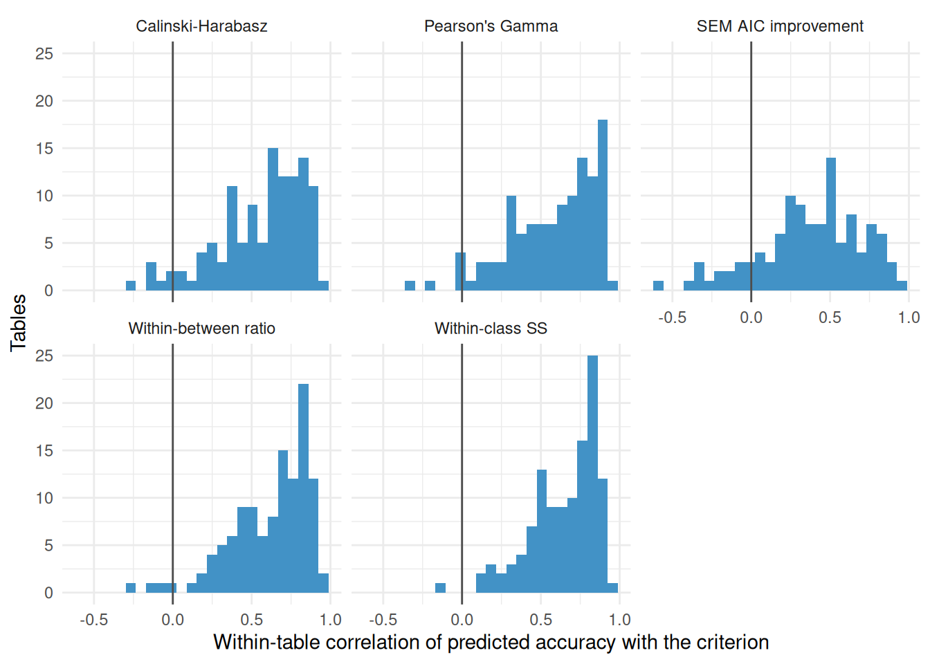
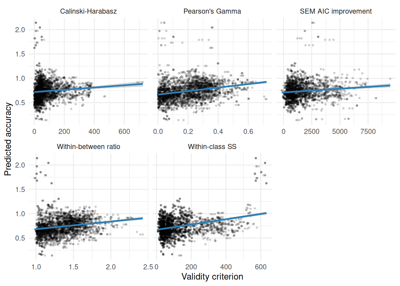
The predictions agree with the criteria about as well as they did in the original study. The mean within-table correlations for within-class sum of squares (0.64), the within-between ratio (0.62), Pearson’s Γ (0.58), and Calinski–Harabasz (0.56) all fall within the published range. The SEM correlation is also positive, but weaker (0.38). As the warning above notes, some of this agreement may reflect the shared basis in correlation.
The number of classes each method identifies may also contribute. Partition-based criteria depend partly on how many classes a partition contains. Table 4 reports the associations between class count and the five criteria.
| Criterion | rho with k |
|---|---|
| Pearson’s Gamma | 0.42 |
| Within-class SS | 0.54 |
| Within-between ratio | 0.48 |
| Calinski-Harabasz | -0.20 |
| SEM AIC improvement | 0.38 |
Methods with higher predicted accuracy tend to identify more classes (mean within-run ρ = 0.29). Four of the five criteria also favor partitions with more classes; Calinski–Harabasz is the exception and favors fewer. Agreement on those four may therefore partly reflect a shared preference for finer partitions. Agreement on Calinski–Harabasz runs against that tendency, so it is not explained by class count.
We retain the published comparisons without adjusting for class count. These associations do not tell us how much of the agreement class count explains.
For every criterion, the pooled correlation is smaller than the mean within-table correlation. The two summaries therefore give different impressions of agreement. The within-table correlations address our question more directly: how do the methods compare for a given dataset?
Q2. Does the best measure vary across tables?
| Method | Calinski-Harabasz | Pearson’s Gamma | Predicted accuracy | SEM AIC improvement | Within-between ratio | Within-class SS |
|---|---|---|---|---|---|---|
| eJaccard | 3% | - | 1% | 8% | - | 1% |
| Podani | 3% | 2% | - | 8% | 2% | 3% |
| Euclidean | 0% | - | - | 25% | - | - |
| Cosine | 1% | 11% | - | 7% | 11% | 7% |
| eDice | 1% | 1% | - | 0% | - | - |
| Correlation | 15% | 63% | 22% | 22% | 69% | 56% |
| ACE | 1% | 8% | - | 5% | 7% | 18% |
| Original Relationality | 1% | - | 1% | 4% | - | - |
| Recursive Relationality | 16% | 9% | 77% | 17% | 5% | 9% |
| Ensemble | 59% | 7% | - | 3% | 7% | 6% |
| Basis | Its share of wins | Top method | Distinct winners |
|---|---|---|---|
| Calinski-Harabasz | 59% | Ensemble | 10 |
| Pearson’s Gamma | 63% | Correlation | 7 |
| Predicted accuracy | 77% | Recursive Relationality | 4 |
| SEM AIC improvement | 25% | Euclidean | 10 |
| Within-between ratio | 69% | Correlation | 6 |
| Within-class SS | 56% | Correlation | 7 |
Recursive relationality has the highest predicted accuracy in 77% of runs, and only 4 measures ever rank first. The models thus recommend the same measure for most of the 117 tables. The differences between these tables and the 10-item, 100-respondent training matrices may help explain this result, as discussed below.
The validity criteria also concentrate, but on a different measure. Correlation ranks first under three of the five criteria: 63% of runs under Pearson’s Γ, 69% of runs under the within-between ratio, 56% of runs under within-class SS. The ensemble ranks first in 59% of runs under Calinski–Harabasz. Only the SEM criterion is widely spread: its leading method, Euclidean, accounts for 25% of runs, and 10 methods rank first at least once. Correlation’s strong showing needs to be read in light of the correlation-based criteria.
The best measure therefore varies across tables, but less than the original study suggested. Even under the most concentrated criterion, a different measure wins in about a third of runs, so no measure is best everywhere. But on four of the five criteria a single measure wins most runs, and three of those favor the measure that the criteria are built to favor. The predictions and the criteria also disagree about which measure that is: the models favor recursive relationality, while the criteria mostly favor correlation.
Class solutions and degeneracy
| Method | median k | median substantive k | median largest class |
|---|---|---|---|
| eJaccard | 3 | 3 | 44% |
| Podani | 4 | 4 | 40% |
| Euclidean | 3 | 3 | 44% |
| Cosine | 5 | 4 | 34% |
| eDice | 3 | 3 | 43% |
| Correlation | 4 | 4 | 33% |
| ACE | 6 | 5 | 32% |
| Original Relationality | 3 | 3 | 43% |
| Recursive Relationality | 4 | 4 | 35% |
| Ensemble | 3 | 3 | 38% |
No run produced a degenerate solution (a single class, or one class holding more than 90% of respondents), and none failed.
The reverse-keying diagnostic
Recovered classes may separate respondents by response polarity rather than by distinct covariance patterns. For each table and method, we assess how closely class membership corresponds to respondents’ alignment with the signs of the first principal-component loadings. We summarize this relationship as the share of variance in PC1 polarity scores explained by class membership (η²).
| Method | Q1 | Median | Q3 | Max | share > 0.5 |
|---|---|---|---|---|---|
| eJaccard | 0.201 | 0.349 | 0.554 | 0.843 | 32% |
| Podani | 0.068 | 0.181 | 0.296 | 0.737 | 5% |
| Euclidean | 0.112 | 0.202 | 0.381 | 0.761 | 9% |
| Cosine | 0.202 | 0.361 | 0.485 | 0.938 | 23% |
| eDice | 0.052 | 0.119 | 0.217 | 0.484 | 0% |
| Correlation | 0.063 | 0.148 | 0.270 | 0.606 | 2% |
| ACE | 0.062 | 0.140 | 0.285 | 0.633 | 2% |
| Original Relationality | 0.030 | 0.076 | 0.162 | 0.492 | 0% |
| Recursive Relationality | 0.051 | 0.160 | 0.335 | 0.790 | 10% |
| Ensemble | 0.071 | 0.196 | 0.351 | 0.757 | 7% |
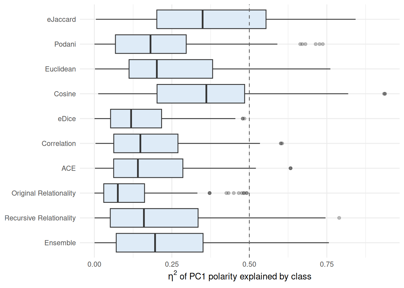
eJaccard and cosine show the strongest associations with response polarity. Their η² exceeds .5 in about a third and a quarter of tables, respectively. This does not establish that the classes lack substantive meaning, but it affects their interpretation. When class membership closely follows response polarity, a high validity score provides limited evidence that the method has identified distinct covariance patterns.
How far the tables are from the training data
Every one of the 198,000 simulated matrices used to train the models had 10 items and 100 respondents. Item count was not among the parameters the authors varied (their Table 3).
| Quantity | Value |
|---|---|
| Items: min | 6 |
| Items: median | 12 |
| Items: max | 37 |
| Items: % at 10 | 12% |
| N: min | 202 |
| N: median | 606 |
| N: max | 2000 |
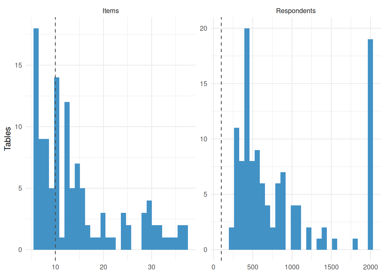
The IRW tables differ from the training matrices in both item count and sample size. These differences may help explain the results, although we cannot establish how much they matter. Two meta-features, PercentOut and intrinsicDimProp, are divided by item count. Others, including VarColPC1 and OverallSD, depend on scale and the number of response categories.
Applying models trained on 10-item, 100-respondent matrices to tables with up to 37 items and 2,000 respondents therefore requires extrapolation. The released materials do not allow us to quantify the resulting prediction error. Simulations covering a wider range of item counts and sample sizes would allow a more direct test of the procedure for these data.
Conclusion
The results largely support Sotoudeh and DiMaggio’s assessments. Predicted accuracy agrees with four of the five validity criteria about as well as it did on the original survey modules. The measures they recommended, recursive relationality and correlation, rank near the top, and Euclidean distance and original relationality rank near the bottom. Support for their broader finding that no measure is best across datasets is weaker: the best measure still varies, but four of the five criteria favor a single measure in most runs, three of them correlation. The prediction models provide less useful guidance: they recommend the same measure for most tables. The narrow simulation design may contribute to this result, but its role remains uncertain. A wider simulation design and clearer documentation of the code issues in Table 1 would help establish when the procedure can guide method selection for item-response data.
Limitations
- The simulated training data were not released, and the fitted models do not retain their model frames. We can compare our tables with the authors’ nine empirical datasets, but cannot compare them directly with the data used to train the models.
- The noise-assumption models cannot be loaded, so we do not test the claim that the ensemble’s advantage grows with error variance.
- The released code uses Louvain community detection throughout. The authors report that this choice affected performance, so our results are conditional on it.
- The validity criteria are computed from correlations and so favour correlation-based measures, as the authors acknowledge.
- 47 of the 118 sampled tables have no construct tag, so comparisons by construct type rest on fewer tables.
- One sampled table,
sd3ypl_klimczak_2019_sd3, could not be analysed (see Corpus), so the results are based on 117 tables, not - We excluded tables with more than 50,000 respondents because of download costs. This practical restriction limits the sampling frame.
- Two 40-item tables (
hexaco_ashton_2014_candhexaco_ashton_2014_h) were excluded after sampling because of computational costs. At 2,000 respondents, each required about 19 core-hours. We did not replace them because substitutes would have had fewer items, underrepresenting the widest tables. The analytic sample therefore contains at most 37 items per table, making extrapolation from the 10-item training matrices less extensive than the full sampling frame would permit.
Appendix: implementation sensitivity
| reading | min | median | max | below 0 | above 1 | undefined |
|---|---|---|---|---|---|---|
| pct_cells | 0.141 | 0.720 | 2.142 | 0% | 6% | 0 |
| positional | 0.726 | 1.871 | 6.334 | 0% | 97% | 0 |
| primary | -2.242 | -0.218 | 1.030 | 62% | 0% | 0 |
| rk_corrected | -2.153 | -0.191 | 1.027 | 61% | 1% | 27 |
Table 9 compares predicted accuracy under four specifications: the released PercentOut formula (primary), the cell-proportion PercentOut used in the main analysis (pct_cells), the corrected OverallRightKurt (rk_corrected), and the released positional matching of coefficients to meta-features (positional). Under the released PercentOut formula, 62% of predictions fall below zero; under positional matching, 97% exceed one.
These choices substantially affect which measure is selected. Relative to pct_cells, the same measure ranks first in only 30% of tables when we use the released PercentOut calculation. Agreement falls to 18% when OverallRightKurt is corrected and to 1% when coefficients are matched by position, as in the released code.
Acknowledgments
We thank Ramina Sotoudeh for her helpful comments on this analysis.
Reproducibility
Source code for this page: plenitude_replication.qmd · plenitude_replication_compute.R · plenitude_lib.R · plenitude_data_prep.R · plenitude_sample.R · plenitude_collate.R
Results were computed on October 23, 2026. To regenerate the analysis, run the following commands from the project root:
# 1. Draw the corpus (deterministic given the seed)
source("analysis/plenitude_sample.R")

# 2. Fetch, fit and collate. Skip-if-exists at the table x replicate level,
#    so the run is resumable. Needs REDIVIS_API_TOKEN for the fetch stage.
#    ~140 core-hours; PLENITUDE_WORKERS controls parallelism. Stops before
#    fitting if check_criteria_orientation() fails.
source("analysis/plenitude_replication_compute.R")

# 3. Re-render this page
quarto::quarto_render("analysis/plenitude_replication.qmd")References
Boutyline, Andrei. 2017. “Improving the Measurement of Shared Cultural Schemas with Correlational Class Analysis: Theory and Method.” Sociological Science 4: 353–93. https://doi.org/10.15195/v4.a15.
Goldberg, Amir. 2011. “Mapping Shared Understandings Using Relational Class Analysis: The Case of the Cultural Omnivore Reexamined.” American Journal of Sociology 116 (5): 1397–436. https://doi.org/10.1086/657976.
Sotoudeh, Ramina, and Paul DiMaggio. 2021. “Coping with Plenitude: A Computational Approach to Selecting the Right Algorithm.” Sociological Methods & Research 52 (4): 1838–82. https://doi.org/10.1177/00491241211031273.